Sovereign Intelligence Infrastructure Under Disruption

Digital Twins, Space–Ground Computing & Assured Multi-Agent Autonomy
Joint observation, computation and authorised intervention under partial observability, disruption and resource constraints.
Abstract
A distributed intelligence system can predict a disruption accurately and still choose an ineffective, unauthorised or physically infeasible response. Its observations may be confounded by previous interventions, its agents may repeat one source, and its most capable processor may be unavailable when the decision must be made. We investigate how observation selection, computation placement and authorised intervention should be designed as a joint decision problem under partial observability, adversarial information and constrained resources.
We propose an architecture that maintains four coupled representations: a causal model of the operational process; an evidence graph recording measurement ancestry and uncertainty; a physical model of computation, communication and recovery; and an authority model governing executable actions. The planner selects information and computation according to their expected contribution to a timely intervention. A separate execution mechanism checks scope, evidence validity, resource feasibility and recovery conditions. Model disagreement, missing industrial dependencies and uncertain fault mechanisms remain visible in the decision rather than being compressed into a single confidence score.
The study combines a critical synthesis of research available by February 2018, formal arguments and reproducible computational exercises. In an exact confounding example, the observed failure-rate difference is positive 17.34 percentage points although the specified causal effect is a reduction of 12 points. Ten repetitions of one likelihood ratio move a naïve posterior from a justified 8.33% to more than 99.99999%. A finite joint policy search over 48 resource and authority configurations yields mean net utility of 1.1795, compared with 1.1142 for the best feasible one-observation policy and 1.0384 for a feasible information-greedy policy. The joint policy also acts more often on false positives, making the consequence weights material to its advantage. Two industrial networks with identical supplier and customer totals produce 2 and 22 units of critical final output under the same specified disruption. A nominal 95% prediction interval covers only 61.43% of observations after the tested distribution shift.
These results identify mechanisms and boundaries within explicit models. The proposed validation programme connects them to hardware, causal interventions, authorised cyber remediation and operational recovery. Conditional scenarios through 2040 examine advances in multimodal inference, quantum-assisted navigation and photonic acceleration without treating component capability as a system guarantee. Our principal conclusion is that useful intelligence is the ability to improve an outcome through a justified, timely and controllable action while preserving the option to recover.
Keywords: causal digital twins; active sensing; space computing; evidence provenance; autonomous agents; supply networks; rare events; sovereign execution.
Contents
1 Research question and contribution
The decision problem
We investigate a single question: how should a distributed intelligence system jointly select observations, allocate computation and execute authorised interventions when its operating environment is partially observed, adversarial and resource-constrained? The question concerns the complete sequence from acquiring evidence to verifying an external effect. A forecast is an intermediate product. Its operational value depends on whether an available action can improve an outcome before the relevant opportunity expires.
Consider a disruption involving a port, a regional substation and a supplier of specialised industrial components. Reduced activity in an image may indicate physical damage, a planned shutdown, loss of electrical supply, missing inputs or a deceptive presentation. A terrestrial diagnostic might distinguish these explanations more quickly than another satellite image. Processing the image aboard a spacecraft may save transmission time but consume battery reserve needed during eclipse. A repair agent may identify an appropriate configuration change yet lack permission to apply it to a particular controller. Restoring the controller may have little effect if the essential supplier remains unable to produce. Each decision therefore changes the value and feasibility of the others.
This coupling is the research problem. Treating sensing, inference, computing and action as independently optimised services can produce a chain in which every component meets its local benchmark while the intervention arrives late, relies on duplicated evidence or violates a physical constraint. A useful system must preserve the relationships between evidence, state, authority and consequences throughout that chain. We consequently take the policy over time, rather than a prediction or a model, as the unit of analysis.
The scope is infrastructure continuity, contested logistics, environmental observation and authorised cyber remediation. These applications can involve deliberate deception and compromised devices without making every anomaly an adversarial act. An anomaly score is not evidence of motive, culpability or hostile intent. Our causal variables concern observable system states and operational outcomes. Decisions affecting people require their own substantive authority and evidence, which cannot be obtained by relabelling an infrastructure forecast.
What sovereignty requires
We use sovereignty of execution to mean the practical ability of an accountable operator to control the identities, keys, updates, tools, computation and recovery processes required for a specified mission over a specified duration. Data location alone cannot establish that control. A locally hosted model may depend on an external identity service, licence server, update channel, accelerator firmware or recovery key. Conversely, a federated service may preserve bounded operational independence through explicit delegation and tested recovery procedures.
This definition is deliberately operational. It asks which decisions remain executable when named dependencies disappear, which actions remain prohibited when an agent is compromised, and how control is restored after an incident. It does not require technological autarky. Dependence becomes a design variable whose effect can be measured through disruption tests, recovery time and the scope of authority retained locally.
Contributions and standards of evidence
Our contribution is an integrated research architecture and a set of constructive tests. We connect causal identification, decision-relevant sensing, correlated evidence, physical scheduling and bounded authority in one model of action. We specify why particular combinations fail, how a proposed control addresses the failure, and what evidence would be needed to support deployment. We do not treat the established foundations of causal inference, distributed consensus or access control as inventions of this study.
The analytical contribution has three parts. First, it separates uncertainties that demand different remedies: missing physical state, unidentified intervention effects, dependent evidence and unavailable resources. Second, it makes recovery a constraint on present decisions, because an apparently useful action may consume the ability to return to a controllable state. Third, it constructs counterexamples and a finite policy comparison whose assumptions and calculations can be reproduced independently.
The numerical exercises are synthetic and specified in full. They demonstrate logical and computational mechanisms, including confounding, evidence duplication and resource-dependent policy changes. They do not estimate the performance of a deployed constellation or an operational intelligence service. The proposed empirical programme addresses that additional question through independent measurement, controlled interventions and end-to-end fault trials. Maintaining this distinction is necessary for the architecture to be assessable: a derivation, a simulation and a field observation justify different conclusions.
2 Research method and foundations
An evidence horizon and a constructive method
We use current data to establish the scientific and engineering basis of the architecture and to develop conditional scenarios through 2040. A scenario specifies mechanisms, assumptions and tests that could support future capability. It is not a measurement of a system that has not been built. Numerical values introduced by this study are identified as parameters or calculated consequences of a specified model.
Our method proceeds from assumptions to interfaces, counterexamples and tests. We begin by identifying the assumptions under which a subsystem claim is valid. We then examine whether neighbouring subsystems supply what that claim requires. Where they do not, we construct a failure case. Finally, we propose a control and an evaluation capable of distinguishing the controlled system from a simpler feasible alternative. This structure prevents an attractive architecture diagram from substituting for an argument about behaviour.
Digital twins offer an important starting point. Glaessgen and Stargel (2012) describe the integration of simulation, health information and operational history for aerospace vehicles. For intervention selection, we require a further distinction between fitting an observed trajectory and identifying what would happen under a changed decision. Pearl (2009) provides the causal framework for that distinction. A fitted simulator can remain causally wrong when historical operators used information absent from its data.
The control problem also has a long foundation. Partially observable decision processes formalise planning when the state must be inferred from observations (Kaelbling, Littman and Cassandra, 1998). Robust dynamic programming addresses ambiguity about the transition model, subject to structural conditions on the uncertainty set (Iyengar, 2005). We extend the state description to include resource availability, evidence ancestry and authority validity. This extension changes the feasible policy set; it does not remove the computational difficulty of general partially observable planning.
Table 1 Foundations and additional integration obligations
| Foundation | Established contribution | Obligation in this study |
|---|---|---|
| Causal inference | Distinguishes observation from intervention | Record hidden decision information and identification conditions |
| Partial observability | Plans from uncertain state and delivered evidence | Include authority and physical resources in the decision state |
| Information gathering | Selects informative observations | Evaluate delivery time and intervention value |
| Robust fusion | Handles specified correlation and fault models | Retain shared ancestry and common failure exposure |
| Distributed systems | Coordinates replicated state under faults | Separate agreement from evidence truth |
| Spacecraft engineering | Models power thermal and communications limits | Check the complete workload and feasible continuation |
| Security and assurance | Constrains access and establishes conditional guarantees | Check every external effect and test clean recovery |
Comparing complete policies
A credible comparison must give competing policies the same observation opportunities, resource constraints, authority scope and intervention objective. A method that observes immediately cannot fairly be compared with one that is forced to wait for a contact window. A policy that acts outside its authority is not a faster version of an authorised policy. A policy that abstains on every difficult case may avoid errors while providing no useful service. We therefore report both useful intervention and the consequences of action, including false-positive actions and delay.
The finite search in Chapter 14 deliberately contains its one-observation comparator. Its non-inferiority in the specified objective consequently follows from the search space as well as the calculations. The informative findings are the magnitude of differences, the conditions under which the selected action changes, and the trade-offs that the objective exposes. The experiment cannot establish universal superiority over every scheduling or sensing method.
We distinguish three types of research assertion. An analytical assertion follows from stated assumptions and can be challenged by examining a proof. A model result follows from a complete executable specification and can be challenged by changing parameters or reproducing the computation. An empirical assertion requires observations from the relevant system and an account of measurement error, selection and uncertainty. Architecture review should reject substitutions between these categories, particularly when a mathematical guarantee is being used to imply field reliability.
A falsifiable integration programme
The architecture is successful only if its additional machinery improves a relevant combination of mission benefit, failure exposure and recovery. Provenance, for example, is useful when it prevents double-counting or enables rapid invalidation of contaminated assessments. It is not sufficient that every database row has a source label. A resource model is useful when it predicts whether useful output will arrive and whether the system can survive the remainder of the mission. Agreement between scheduling software and a simulator sharing the same error is weak evidence.
We therefore retain simple baselines throughout the study. These include one-observation decisions, information-greedy sensing, centralised scheduling when connectivity permits it, fixed safe modes and deterministic access controls. The integrated system must justify its complexity against such alternatives. Where continuous communications, ample power and stable evidence make a central design adequate, decentralisation has no inherent scientific advantage.
3 Formalising the joint decision problem
State history and action
Let the physical state include infrastructure condition, inventories, vehicle states, network topology and any latent causes relevant to the outcome. Let the resource state include battery energy, thermal state, memory, available processors, orbital phase and communications opportunities. Let the authority state include current identities, delegations, policy versions, revocations and expiry times. The delivered history contains observations that have actually arrived, their acquisition times, processing history and the decisions previously taken.
Acquisition time and delivery time are different variables. A recent arrival can describe an old physical state. A high-quality observation can be useless if it arrives after the intervention window. A processor can finish a computation that cannot be transmitted, decrypted or validated in time. A policy must therefore operate on delivered history and available resources, while predicting the consequences of pending observations and unfinished workloads.
We represent uncertainty using a belief over physical state together with a set of plausible causal and fault models. Where a calibrated probability distribution is justified, expected utility can be evaluated under it. Where evidence supports only bounds or several competing structural models, the policy must preserve that ambiguity. Assigning precise probabilities to unknown industrial links merely to satisfy an optimiser creates apparent precision without additional knowledge.
Actions comprise observation requests, workload placement, communications scheduling, interventions, deferral and recovery. An observation action may include a trajectory change or pointing manoeuvre. A computation action may allocate an accelerator, choose an approximation or create a checkpoint. An intervention may change an equipment setting, reserve inventory or apply an authorised software repair. These actions compete for time, resources and future options.

Equation 1 Joint policy objective under model ambiguity. Benefits and costs are evaluated only over admissible policies.
Here Πadm contains policies satisfying the hard constraints, M is a declared set of admissible models, and the costs include observation, computation and intervention consequences. The finite horizon H reflects a mission or decision window. The expression is a research formulation rather than a claim that the general problem is efficiently solvable. The computational study restricts the action catalogue and depth so that every feasible candidate can be enumerated.
Constraints that cannot be purchased with reward
Authority and specified physical safety conditions are constraints on admissibility. They cannot be traded away because a model predicts sufficient benefit. Within the admissible set, the operator may explicitly trade observation cost, intervention burden, delay and residual operational loss. This separation is important when a learned planner discovers that a prohibited action would be effective. The proposed action may be informative for a human decision, but it remains non-executable under the current authority state.
Recoverability is also a state-dependent condition. A useful workload that leaves insufficient energy for safe hold is inadmissible under a mission requiring that hold. A software change that destroys the only clean recovery path is inadmissible under a contract requiring rollback. The relevant test concerns a physically reachable and authorised continuation, rather than the presence of a command called “recover”. A successful acknowledgement is not evidence that the promised state was reached.
The ambiguity set requires particular care. If an unknown supplier relationship is fixed during the mission, the model must retain it as a persistent latent variable. Allowing an adversary to replace that relationship independently at every time step may create an excessively pessimistic and internally inconsistent problem. Conversely, applying a robust Bellman recursion to an uncertainty set that lacks the necessary rectangularity can produce an invalid decomposition (Iyengar, 2005). We retain persistent model variables or evaluate whole scenarios where that structure is material.
Risk allocation and model validity
A constraint violation probability is meaningful only relative to the model under which it is calculated. Suppose the probability that the declared model family fails to cover the relevant situation is bounded by β. Suppose the covered model supplies conditional bounds εt for defined failure events along the policy. A union bound yields a mission-level statement without assuming independence.

Equation 2 Conditional mission risk accounting. β bounds model non-coverage; ε terms bound declared failures within the covered models.
The bound is conservative and depends on defensible event definitions. It does not justify summing nominal confidence levels whose meanings differ or whose validity is unknown. If β cannot be estimated or bounded, the resulting claim remains conditional on model adequacy. The architecture must then expose the condition and provide a response to evidence that the model is no longer suitable.
Shared dependencies must remain visible. A navigation fault can simultaneously corrupt image registration, the inferred location of damage and the safety envelope of a repair vehicle. A common clock error can invalidate both evidence freshness and authority expiry. Treating these failures as independent makes the aggregate assurance stronger on paper precisely when the actual system has a common point of failure. We therefore connect risk accounting to the evidence and dependency graphs used during operation.
4 Causal digital twins and interventions
Forecasting under a historical decision process
Historical data describe outcomes under historical decisions. Those decisions may have depended on inspection notes, local experience, private communications or signals that were never recorded. A predictive model can exploit the association between intervention and failure while learning the wrong sign for the intervention effect. In infrastructure operations, maintenance is often directed towards assets already suspected of being at risk. Higher failure among maintained assets does not establish that maintenance caused the failures.
A causal twin must therefore specify the intervention, outcome, population, time horizon and comparison policy. It must distinguish variables observed before the decision from variables caused by it. Adjusting for a post-intervention variable can remove part of the effect or introduce selection bias. Omitting a pre-decision variable used by the operator can leave confounding. More accurate prediction of the observed outcome does not resolve either problem (Pearl, 2009).
Under consistency, adequate overlap and sufficient adjustment variables Z, an intervention mean can be identified by averaging the conditional outcome model over the target distribution of Z. Each assumption has an operational interpretation: the treatment definition must be meaningful, both relevant decisions must occur in comparable situations, and the recorded variables must block the relevant confounding paths.

Equation 3 Adjustment formula under consistency positivity and sufficient adjustment variables.
For sequences of interventions, the problem is more demanding. A variable influenced by an earlier decision may also affect a later decision and the outcome. Robins (1986) provides a foundation for analysing such time-varying treatment and confounding. Doubly robust off-policy evaluation can protect against specified nuisance-model errors, but it does not recover information about hidden confounders merely by combining two estimators (Jiang and Li, 2016).
A sign reversal with completely specified counts
Consider 10,000 assets divided into 2,000 high-risk and 8,000 low-risk cases. The intervention is applied to 1,800 high-risk cases and 800 low-risk cases. In the specified model, high-risk failure probability falls from 0.80 without intervention to 0.40 with intervention. Low-risk probability falls from 0.10 to 0.05. The aggregate treated group has 760 failures among 2,600 cases, while the untreated group has 880 failures among 7,400 cases.
The observed treated failure rate is 29.23%, compared with 11.89% for untreated cases. The observed difference is therefore positive 17.34 percentage points. Applying the intervention to the full population instead gives expected failure probability 12%, compared with 24% if nobody is treated. The specified average causal effect is negative 12 percentage points. The sign reversal arises entirely from the allocation of treatment towards high-risk cases.
If the risk variable were absent from the records, this causal effect would not be identified by the treatment and outcome table alone. Under consistency without additional identifying assumptions, the potential-outcome bounds permit an average effect between −27.2 and +72.8 percentage points. Appendix A derives these bounds following the logic of partial identification (Manski, 1990). The width is useful information: it states that the available records support very different intervention consequences.
Transport and changing operating conditions
An effect identified at one site may not transport to another. Equipment age, environmental exposure, repair practice and supply constraints can change the mechanism through which an intervention works. The architecture therefore stores the target population and the assumptions required to transport an effect, rather than treating every measured benefit as a universal property of the action. Data fusion and transport require a causal account of which mechanisms differ across environments (Bareinboim and Pearl, 2016).
Invariant prediction offers a related way to examine whether a proposed relation persists across environments (Peters, Bühlmann and Meinshausen, 2016). Persistence can support a causal hypothesis under its assumptions; it does not establish invariance under every future intervention or adversarial change. A relation observed across normal weather regimes may fail when a supplier is deliberately disconnected or when operators change their maintenance policy.
We consequently separate three questions in the twin. State estimation asks what is happening now. Effect estimation asks how a defined intervention changes an outcome. Transport asks whether that effect applies under the present operating conditions. High confidence in one answer does not substitute for evidence about the others. The separation also improves active sensing: an additional inspection may reduce uncertainty about state while leaving the intervention effect unidentified.
Learning through bounded intervention
Where causal ambiguity is consequential, the preferred next observation may be an authorised experiment. A reversible change to a non-critical subsystem, applied under controlled conditions, can distinguish mechanisms that passive observation cannot separate. The experiment must preserve essential service and a recovery path. Where randomisation is infeasible, a credible natural experiment or design-based comparison may still provide information, but its identifying assumptions must be tested against the operational process.
The decision record should retain the estimand, comparison policy, outcome horizon, identification assumptions and evidence versions. It should also record why the chosen action remains acceptable across plausible effects. When the effect is only bounded, a conservative action can be selected if it improves outcomes throughout the supported range. Otherwise, deferral, a narrower intervention or additional evidence may be the rational policy. This is an explicit decision under uncertainty rather than an unexplained refusal to act.
5 Active sensing and observability
Selecting information for a decision
The value of an observation is the improvement it can make to an available decision after accounting for acquisition cost, delay and the resources consumed. A more accurate observation can have lower value if it arrives after the action window. An observation that reduces uncertainty about an irrelevant variable can have negligible value. An expensive diagnostic can be valuable when it determines whether an otherwise unacceptable intervention becomes justified.
The observation catalogue should describe the hypotheses each measurement can distinguish, the state on which its likelihood depends, its acquisition geometry, its expected delivery time and its resource requirements. For a satellite image, these include pointing, illumination, cloud or obscuration, registration and transmission. For a terrestrial diagnostic, they include sensor health, access and sampling conditions. For a cyber observation, they include permission, system load and the possibility that the observed service controls the evidence returned.

Equation 4 One-observation value. V is the best permitted intervention or abstention value; h r and t are delivered history resource state and time. Primed quantities denote completion and C is acquisition cost.
The expression evaluates an observation at its completion state. The value function includes the best permitted intervention or abstention, so the calculation can prefer no observation. Resource opportunity cost enters through the changed state as well as any explicit acquisition cost. The same energy cannot simultaneously process an image and preserve the reserve required for another task. Comparing observation values without that coupling can recommend an infeasible collection schedule.
Information gain is not sufficient
Entropy reduction is a useful intermediate objective when its relationship to the decision is established. It is not generally equivalent to expected intervention value. A sensor that distinguishes two harmless causes may have high information gain and little operational benefit. A less informative sensor may identify the one condition under which a low-cost protective action prevents substantial loss.
Greedy observation selection has theoretical support in important structured settings. Near-optimal sensor placement for Gaussian processes and adaptive submodularity provide examples (Krause, Singh and Guestrin, 2008; Golovin and Krause, 2011). Their assumptions must be checked. Suppose two independent fair binary variables U and V jointly determine a hazard H through exclusive-or. Observing U alone or V alone provides no information about H, while observing both determines it exactly. The marginal value of the second measurement rises after the first. This simple construction violates the diminishing-returns intuition that would justify a generic greedy guarantee.
Physical observation planning adds further constraints. A robot may have to travel to acquire information, and that travel changes risk, energy and future access. Sampling-based information-gathering methods address this interaction between geometry and informative measurements (Hollinger and Sukhatme, 2014). A space–ground system adds discontinuous contact windows and workload completion times. The relevant observation action is therefore a complete acquisition-and-delivery plan rather than a sensor name.
Observability and deceptive measurements
Observability concerns whether the observations can distinguish relevant states under the model. A narrow posterior produced by a strong prior does not establish physical observability. Repeated images of the same obscured component may reinforce the prior without supplying new evidence. A system should identify which state differences remain unresolved and whether they would change the selected intervention.
Secure estimation under adversarial corruption provides conditions for reconstructing state when some sensor channels may be attacked (Fawzi, Tabuada and Diggavi, 2014). Such conditions depend on the system dynamics, redundancy and the permitted corruption model. Adding sensors is not sufficient if all channels share a vulnerable clock, calibration source or communications path. The architecture must distinguish channel count from independent information and independent failure exposure.
Multisensor image fusion also depends on alignment and compatibility. Resolution, observation geometry and acquisition time influence what a fused product can claim (Pohl and van Genderen, 1998). A thermal anomaly and a visible change do not necessarily concern the same physical component unless registration uncertainty is controlled. If location is uncertain, the intervention target must remain uncertain too. A confident assessment attached to the wrong asset is operationally misleading even when the classification itself is correct.
Generated imagery and measurement gaps
A generated image can be useful for simulation, hypothesis construction or communication. It cannot fill a missing physical observation merely because it is visually plausible. If an obscured route is reconstructed from a model prior, the clear route in the generated product is not evidence that the route is clear. The product should retain its dependence on the original observations and the model that generated it.
The planner should respond to a consequential measurement gap by acquiring a discriminating observation, choosing an action safe across the unresolved alternatives, or deferring the intervention. This treatment becomes increasingly important as synthesis improves. Visual realism can reduce the human visibility of uncertainty without reducing the uncertainty itself. The evidence graph and action guard must preserve the distinction even when an agent’s natural-language explanation does not.
6 Adversarial evidence and correlated assessments
Evidence ancestry as an operational object
An evidence graph records measurements, transformations and conclusions as distinct objects. Each measurement retains its source, acquisition time, location or frame, calibration, content digest and delivery history. Each transformation retains its software and model version, inputs and relevant parameters. Each assessment identifies the observations on which it depends. The graph also records shared dependencies such as a clock, navigation solution, training corpus or common preprocessing service.
Cryptographic authentication establishes that a message came from a particular key holder and has not been altered within the protected channel. It does not establish that the sensor was correctly calibrated, the source was independent or the reported event occurred. A compromised but validly authenticated sensor can supply consistent false data. A legitimate analyst can repeat another source without recognising the dependence. The graph must support both cases without confusing authenticity with truth.
Evidence confidence should therefore be propagated through dependence, not accumulated by counting reports. Ten agents repeating one image are ten processing paths from one observation. They may expose different errors or extract different features, but their agreement cannot be treated as ten independent physical measurements. Model diversity can be useful, yet a shared training distribution or common preprocessing fault can still dominate the combined assessment.
Duplication and falsely narrow uncertainty
Suppose a hazard has prior probability 1% and one observation has likelihood ratio 9. Bayes’ rule yields a posterior probability of 8.33%. If ten agents repeat that observation and the system multiplies the same likelihood ratio ten times as though the reports were independent, the posterior exceeds 99.99999%. No additional physical evidence has been acquired. The confidence increase is a bookkeeping error.
The same problem appears in continuous estimation. For ten equally precise estimates with pairwise correlation ρ, the variance of their mean is larger than the independence calculation by a factor of 1 + 9ρ. The corresponding effective independent sample size is 10 divided by that factor. At correlation 0.8, ten reports contain the variance-reduction equivalent of approximately 1.22 independent reports. A nominal 99% Gaussian bound calculated under independence then has actual exceedance probability of about 36.84% under the specified correlated model.
Covariance intersection provides a conservative method for combining estimates when cross-correlation is unknown, under suitable consistency of the input estimates (Julier and Uhlmann, 1997). It does not repair a shared unmodelled bias or make an adversarial input covariance truthful. The selection of a conservative fusion rule must therefore accompany a model of what can be wrong with the sources, rather than replace it.
A limit on synthetic corroboration
Let X be the physical quantity of interest, Y the measured data, θ a fixed trained model and R fresh random input independent of X given Y and θ. A generated representation G is a function of Y, θ and R. Conditional on those inputs, generating G does not create additional information about X.

Equation 5 A generated representation supplies no additional conditional physical information under the stated independence assumption.
This follows from conditional independence and the data-processing principle (Cover and Thomas, 2006). It does not imply that computation is useless. A model can extract useful information from a complex observation that a constrained downstream agent could not readily interpret. The model can also introduce prior knowledge encoded in θ. The claim is narrower: the generated output is not an additional independent witness to the same physical event. Generative modelling makes this distinction operationally relevant (Goodfellow et al., 2014).
If the generator receives a new physical measurement, the conditioning set changes and the conclusion must be reconsidered. The evidence graph should show that new measurement explicitly. Otherwise, an image-to-text-to-image chain can manufacture apparent source diversity while preserving the same original uncertainty. Counting the final products as separate corroboration would reward transformations rather than observations.
Contamination and invalidation
When a source is found to be compromised, invalidation must follow its descendants. These include cached features, map updates, causal estimates, summaries, agent memory, plans and generated imagery. Deleting the original message leaves the operational consequences intact if its descendants remain trusted. A proposed intervention based on an invalidated assessment must be cancelled or re-evaluated against clean evidence before execution.
Recovery requires a known-clean checkpoint and a way to replay valid observations without reintroducing the contaminated branch. The system must also distinguish an evidence correction from a physical compensation. Reversing a mistaken configuration change can itself require authority and can have consequences that differ from those of the original change. Provenance supports identifying what needs review; it does not make every external effect reversible.
The performance cost of this design should be measured. Recording lineage consumes storage and bandwidth. Conservative dependence handling can reduce apparent confidence and delay action. Broad invalidation can remove useful information alongside contaminated material. The evaluation must quantify whether the reduction in harmful decisions justifies these costs under the mission’s loss function. An assurance mechanism that cannot be exercised under realistic load remains an architectural proposal.
7 Physical limits of space and ground computation
Computation is a scheduled physical activity
Space computing must be evaluated as part of a spacecraft, not as an isolated processor. Orbital geometry determines observation and contact opportunities. Eclipse changes power availability. Thermal rejection constrains how long a workload can run, and battery reserve constrains what remains possible afterwards. Attitude changes made for imaging or communications can alter power generation and thermal exposure. Radiation can interrupt computation or corrupt state. These effects jointly determine whether an inference result will be available and usable at the required time.
The small-spacecraft technology survey compiled by NASA (2015) provides a relevant engineering baseline for power, communications, computing and other subsystems. The central architectural implication is that component specifications cannot simply be combined at their individual maxima. Peak processor performance may be unavailable under the spacecraft’s thermal conditions. Peak communications rate may occur only during a limited geometry. A scheduling model must describe the simultaneous operating state and its transitions.
We describe a workload by its input volume, permitted approximation, processing duration, power demand, heat dissipation, intermediate storage, output size and expiry. Its completion condition includes delivery and validation, not merely the end of arithmetic. Ground computing has its own queues, energy constraints, connectivity and authority dependencies. Moving work to the ground can improve processing capability while making the result dependent on transmission and a remote service that may be unavailable.
Energy and thermal feasibility
A simplified battery model distinguishes charging and discharging efficiencies. Over an interval measured in seconds, net positive generation is multiplied by charging efficiency and net demand is divided by discharging efficiency. Energy must remain above the required reserve throughout the workload, not just at the sampled endpoints. Excess charging is curtailed at battery capacity.

Equation 6 Battery energy increment. Positive-part notation selects charging or discharging and the factor 3600 converts watt-seconds to watt-hours.
Here positive-part notation selects charging or discharging, power is measured in watts and energy in watt-hours. A complete flight model would also account for peak current, voltage, temperature-dependent performance, ageing and battery qualification. The simplified model in Chapter 14 is sufficient to demonstrate coupling between job selection and reserve, but it is not a battery qualification model.
Thermal dynamics introduce memory. A workload that is feasible from a cool initial condition may be infeasible after another task has heated the structure. A single-node representation balances dissipated and externally absorbed heat against radiative rejection. The fourth-power temperature term makes the balance nonlinear even in this reduced representation.

Equation 7 Reduced thermal dynamics. A single node illustrates scheduling dependence but does not replace spacecraft thermal qualification.
CT is thermal capacitance, εA combines effective emissivity and radiating area, and σ is the Stefan–Boltzmann constant. A real spacecraft requires multiple thermal nodes, conductance paths, material properties and attitude-dependent external heat loads (Gilmore, 2002). We use a single node to expose scheduling consequences and retain the need for subsequent thermal qualification. Treating an average power budget as a thermal guarantee would ignore transient heating and local component limits.
Feasibility includes a continuation. We require the selected job to leave enough energy and thermal margin for a specified safe hold through the remainder of the modelled horizon. This prevents the optimiser from borrowing resources from an unmodelled future. More demanding missions would replace safe hold with a reachable communications, navigation or recovery state and verify that continuation under the relevant uncertainty.
Contacts delivery and interrupted workloads
Delay-tolerant networking provides an architectural basis for communication across disrupted or intermittent links (Cerf et al., 2007). For decision scheduling, the contact graph must include time and capacity. A raw-data transfer may need several contacts; a compact inference result may fit in one. A partial transfer may occupy storage without yielding a usable observation. Encryption, authentication and validation consume resources and time after transmission.
An output’s value should therefore be evaluated at the time when the recipient can use it. If an authority token expires before validation finishes, timely radio delivery alone is insufficient. If an observation is stale by the time it arrives, a subsequent prediction step may be required. If the receiver lacks the key or compatible model version needed to interpret the output, the communication schedule has not completed the decision task.
A useful policy can combine compact results with selective raw-data retention. A compact output may support a timely bounded intervention, while retained raw data enables later review or reprocessing. The retention policy must nevertheless account for limited storage and the risk that a compressed result conceals an important failure mode. The choice between raw and processed data is conditional on the decision, the uncertainty model and the available contact schedule.
Radiation faults and recovery overhead
Radiation effects include mechanisms with different persistence and recovery requirements. A transient upset, a latch-up event and accumulated damage cannot be represented adequately by one generic probability that a task fails (Sinclair and Dyer, 2013). Error detection, correction, watchdogs, restart and hardware redundancy address different parts of this fault space. A fault model should specify what is corrupted, how it is detected and which state remains trustworthy afterwards.
Checkpointing trades repeated-work loss against checkpoint overhead. A first-order approximation gives a characteristic interval proportional to the square root of twice the checkpoint cost divided by the failure rate, with more refined treatment available in Daly (2006). For an illustrative checkpoint cost of 30 seconds and a mean interruption interval of six hours, the square-root approximation is about 1,138 seconds, or 19 minutes. These assumed parameters are not a measured radiation rate or an assurance claim.
Restart correctness is separate from restart speed. A checkpoint can contain corrupted evidence, obsolete authority or an incompatible software state. Restoring it can reintroduce a fault or resurrect an expired permission. A clean recovery path therefore needs validated inputs, approved software and current authority, together with a local fallback that does not depend on the failed service. Recovery tests must include those dependencies rather than merely timing process relaunch.
8 Compromised agents and bounded cooperation
Three different failure classes
An autonomous agent can fail by being unavailable, by making an honest but correlated error, or by acting adversarially. These cases require different controls. Replication can improve availability while preserving a common error. Agreement can be achieved among agents sharing the same false premise. An adversarial agent can exploit interfaces, excessive permissions or the trust attached to its outputs even when its own predictions appear accurate.
Byzantine agreement provides foundational results about coordination in the presence of arbitrary behaviour (Lamport, Shostak and Pease, 1982). Practical Byzantine fault tolerance shows how replicated services can maintain agreement under an explicit fault model (Castro and Liskov, 1999). Agreement is valuable, but it is not evidence that an external observation is true. A replicated service can consistently store a false report. The architecture must connect consensus to authenticated state transitions while retaining separate controls for evidence quality and causal interpretation.
Sequence models expand the range of information an agent can process and the plans it may propose. Attention-based modelling illustrates a significant direction in this capability (Vaswani et al., 2017). Neither sequence modelling nor fluent explanation establishes that a proposed action is authorised, causally effective or recoverable. We consequently treat the agent as a proposal-generating component inside an execution architecture, with its access constrained independently of its own interpretation of instructions.
Roles and authority attenuation
We separate observing, assessing, proposing, approving and executing. A role may be implemented by software or an accountable human process, but the separation concerns permissions and evidence, not labels. An observation agent may read a particular sensor stream without changing it. An assessment agent may produce hypotheses without writing verified facts into the shared state. A planning agent may propose a workflow without minting the authority needed to execute it.
Delegation must attenuate authority. A subordinate agent can receive a narrower resource scope, a smaller parameter range, a shorter duration or a smaller action budget. It cannot enlarge those limits by generating a persuasive explanation or by asking another agent to act on its behalf. The tool boundary checks the principal and the complete delegation chain, so a cascade of agent messages cannot manufacture new rights.
The same principle applies to shared memory. An agent’s output should enter as a claim with ancestry and status. It should not automatically become a verified relation in an ontology or a high-trust instruction for the next agent. Schema validation prevents malformed records but does not establish their truth. Evidence checks, conflict handling and versioned acceptance are required before a claim can support an external effect.
Robust aggregation and its limits
Resilient consensus depends on graph structure and the distribution of faulty participants (LeBlanc et al., 2013). A bound on the total number of compromised agents differs from a bound on compromised neighbours at each node. Changing membership, allowing duplicated identities or concentrating compromised agents around a critical node can invalidate the guarantee. Fault assumptions must therefore be expressed in the actual communications and authority topology.
A simple scalar exercise illustrates what robust aggregation can and cannot do. Five honest values are 0.08, 0.09, 0.10, 0.11 and 0.12; two compromised values are 0.99. The arithmetic mean is approximately 0.3543. Removing the two largest and two smallest values leaves a mean of 0.11. Under a bound of at most two arbitrary values among seven, this trimmed result lies within the honest range. If every honest value shares an unmodelled bias of 0.57, the same trimming rule returns 0.68. Resistance to outliers has not established calibration.
For a scalar set with at most f arbitrary values and more than 2f entries, trimming f values from each end removes any arbitrary value lying outside the honest range. The retained average therefore remains within that range. This finite-sample range argument does not establish distributed convergence, vector consistency or the correctness of the honest values. Those are additional claims with additional assumptions.
Containment as a performance trade-off
Containment includes scoped credentials, bounded tool interfaces, resource quotas, isolated execution, rate limits and explicit acceptance of shared-state changes. The objective is to prevent one compromised agent from changing the conditions under which all other agents operate. A malicious observation should not grant access, a malformed plan should not become executable code, and an agent’s self-assessment should not be the sole acceptance test for its own output.
Containment can reduce performance. Quarantining a sensor agent removes coverage. Requiring an independent check adds latency. Restricting shared memory can limit useful coordination. The appropriate comparison measures both the prevented cascade and the loss of service under benign conditions. A design that blocks every action is contained but operationally empty. The computational and empirical evaluations must therefore include useful completion, false action, time to isolate and time to restore service.
Re-entry after quarantine requires more than a new process identifier. The system must establish that credentials, software, state and dependencies have been restored to an acceptable condition. Historical outputs from the compromised interval remain subject to review. A physical effect that occurred during that interval may require a separately authorised compensating action. Rejoining the communications graph cannot itself establish that the external environment has recovered.
Authorised cyber remediation
Automatic software repair and binary analysis provide useful research foundations for bounded cyber tasks (Le Goues et al., 2012; Shoshitaishvili et al., 2016). Within this architecture, an agent may inspect an authorised system, identify a defect and construct a candidate repair in an isolated environment. Acceptance requires evidence that the repair addresses the defect, preserves required functionality and can be deployed within the current operating constraints.
The repair generator cannot be the sole oracle for success. Tests derived from the same mistaken model can approve an ineffective or harmful change. Independent regression, security and deployment checks are therefore separate activities, with their own evidence and authority. A technically valid patch may still be inappropriate during a critical operational interval. The planner can prepare it while deferring deployment until the resource, service and recovery conditions are satisfied.
9 Sovereignty of execution and recovery
Dependency control beyond data location
The execution dependency graph includes identity providers, certificate authorities, key stores, update channels, model repositories, tool gateways, operating systems, accelerators and recovery services. A system is sovereign for a declared mission only to the extent that the accountable operator can maintain or recover the necessary control under the specified disruptions. This is a property of the dependency graph and operating procedures, not a property of a data-centre address.
The graph should identify minimal sets of dependencies whose loss prevents a required function. A locally available model that needs a remote authentication service for every tool call has a different disruption profile from one with narrowly scoped local credentials. A local update cache can improve continuity while increasing exposure to stale or compromised artifacts. These trade-offs should be tested through removal of the relevant service rather than inferred from an inventory diagram.
The required duration matters. Maintaining bounded inspection for six hours during a communications loss is a different claim from independently rebuilding a damaged system after several weeks. The latter may require clean software, firmware, keys, technical documentation, compatible hardware and trained personnel. The recovery dependency graph can be more restrictive than the runtime graph and must be examined separately.
Enforcing permission at the external effect
Least privilege and complete mediation provide the foundation for execution control (Saltzer and Schroeder, 1975). Attribute-based access control supplies a structured way to evaluate subject, resource, action and environmental attributes (Hu et al., 2014). In our architecture, a command carries a target, operation, parameter bounds, delegation chain, expiry, policy epoch and the evidence version on which the proposal depends.
The execution guard checks these attributes at the point where the external state can change. Checking only when a plan is generated leaves a time-of-check to time-of-use gap. A queued command can outlive its evidence or authority. A retry worker can repeat an action after the original permission has expired. A scheduled task can execute under a different resource state from the one used during planning. Every path to the effect, including retries and recovery workers, must pass the guard.
The guard should have a smaller, more stable specification than the planner. It need not determine whether a complex strategy is globally optimal. It must reliably establish that the requested operation is within scope, currently valid and consistent with the defined execution contract. This reduces the amount of software whose compromise could directly enlarge authority, while preserving the planner’s ability to search among permitted actions.
Disconnected revocation
Immediate global revocation cannot be guaranteed to a disconnected executor that continues to accept previously granted authority without receiving new information. Consider two histories identical at that executor: in one, the issuer has revoked the grant; in the other, it has not. The executor receives no message distinguishing the histories. A decision rule based on its local state must behave identically in both. It therefore cannot both continue correctly in the unrevoked history and enforce the unseen revocation immediately in the revoked history.
This argument is an information limit, related to the constraints on consistency and availability during network partitions (Gilbert and Lynch, 2002). Short leases can bound exposure if clock uncertainty is controlled. Local emergency authority can permit specified protective actions during disconnection. Neither mechanism creates knowledge of an unseen remote revocation. The contract must state whether disconnection leads to expiry, reduced scope, a local safe mode or continued authority for a bounded interval.
Clock failure is part of this contract. An expiry time is ineffective if the executor accepts an arbitrarily stale or manipulated clock. The system should combine trusted time where available, conservative uncertainty bounds and failover rules appropriate to the action. A local stop operation may have different authority semantics from a remote reconfiguration. Treating every action identically can either expose excessive authority or disable necessary protection.
Updates and clean recovery
Update systems need protection against key compromise, rollback and inappropriate combinations of metadata and artifacts. Role separation and survivable key-compromise designs provide a foundation for this problem (Samuel et al., 2010). The relevant architecture must define who can publish, approve and activate software or models, and how a compromised role is replaced without granting the attacker lasting control.
Formal verification can support a narrow trusted computing base. The seL4 work demonstrates the depth of assurance possible for an operating-system kernel relative to a formal specification and its assumptions (Klein et al., 2009). Such a result does not automatically verify the application, device firmware, sensors or operational policy. The system assurance case must show how the verified component’s guarantees are used and where unverified dependencies remain.
Recovery trials should remove the primary identity service, interrupt updates, corrupt a candidate checkpoint and expire previously valid delegations. A successful recovery restores a defined service with valid authority and clean evidence. It must not silently revive permissions that were deliberately withdrawn. The trial should measure both restoration time and the residual functions that remained available during recovery, because continuity and eventual restoration are distinct outcomes.
10 Hidden industrial dependencies
Why aggregate connectivity is insufficient
Production networks transmit disruptions through specific input requirements, inventories and substitution constraints. Network structure can turn local shocks into aggregate fluctuations (Acemoglu et al., 2012). Input specificity affects how disruptions propagate between firms (Barrot and Sauvagnat, 2016). A national or sectoral exposure measure cannot identify every bottleneck relevant to a particular critical service.
Observed supplier and customer totals often leave many compatible transaction networks. An inferred edge should therefore carry a status distinguishing confirmed, probable and merely compatible relationships. A single completed graph can conceal uncertainty that materially changes the predicted disruption. Bayesian network reconstruction offers useful methods for reasoning over incomplete networks, although a method developed for financial exposures does not by itself provide the production dynamics of industrial systems (Gandy and Veraart, 2017).
The twin should maintain a set or distribution of feasible networks consistent with known totals, verified links and sector constraints. Interventions can then be evaluated across those alternatives. If a proposed response succeeds only under one unverified network, the missing relationship becomes a candidate for active investigation. An industrial inquiry may consequently have greater value than an additional broad-area image.
Production requires usable inputs
An inventory count is not the same as a usable input quantity. Material may be reserved, quarantined, in transit, unqualified for a particular production line or dependent on an unavailable tool. A nominal substitute may require certification, redesign or scarce production capacity. These distinctions determine the time at which substitution changes output.
A simple fixed-recipe model bounds production by installed capacity and the least available essential input. The model is appropriate for illustrating bottlenecks when each unit of output requires specified quantities of the listed inputs.

Equation 8 Essential-input production bound for a fixed recipe and usable inventory.
Here qj is output, q̄j is capacity, Ijk is usable inventory of input k, djk is delivered quantity and ajk is the requirement per unit. The expression assumes compatible timing and usable inputs. It omits price adjustment, endogenous demand, labour constraints and substitution unless those mechanisms are represented separately. Those omissions should be tested when they affect the decision rather than hidden inside a generic network weight.
Production and transport interact. Reallocating one supplier’s output can support a critical downstream service while reducing another customer’s production. An objective that maximises total units may differ from one that preserves minimum regional service or a particular critical capability. The selected intervention must therefore state the outcome being protected and the burdens imposed elsewhere in the network.
Identical margins and different disruption consequences
Consider two suppliers and two component manufacturers. In one network, each supplier provides ten units to a different manufacturer. In another, each supplier provides five units to each manufacturer. Both networks have identical supplier totals and identical manufacturer totals. Suppose one supplier is lost for four days. Each manufacturer begins with two units of usable input, has capacity ten per day, and produces a different component. Final assembly needs one of each component and has capacity ten per day.
The concentrated network produces two units of final output over the disruption. The diversified network produces 22. The difference follows from the distribution of the surviving input, not a difference in aggregate pre-disruption flow. A reconstruction method that recovers the margins exactly but selects the wrong topology can therefore be severely misleading for intervention planning.
If substitution in the concentrated network becomes available after two days, cumulative final output rises to 12 units. Immediate substitution yields 22 units. Increasing opening inventories to ten units at each manufacturer yields ten units under continued concentration. These outcomes show why inventory, qualification delay and topology cannot be compressed into a single resilience score. Chapter 14 reports the complete daily accounting.
Information and action under incomplete networks
The appropriate inquiry targets an uncertainty that changes the response. Confirming the supplier of a unique component can be more valuable than refining an already adequate estimate of total sector output. Evidence about qualification time may dominate evidence about nominal spare capacity. The causal twin should calculate the consequence of each unresolved dependency under the candidate interventions and present the decision sensitivity explicitly.
Robust planning across compatible networks can identify actions that preserve critical output despite structural uncertainty. Such planning can also become excessively conservative if the compatible set includes unrealistic networks. The set must therefore be constrained by verifiable information and updated as evidence arrives. An adversarial environment increases the importance of provenance for supplier declarations, inventory reports and claims of substitutability.
11 Rare events and anticipatory detection
Define the event and the opportunity to act
Anticipatory detection requires a defined event, population, observation window and prediction horizon. An alert before an event is useful only if it arrives early enough for a permitted intervention to change the outcome. Lead time should therefore be measured from usable alert delivery to the last effective intervention time, alongside the time to actual event onset. A system can predict an event early in a data file yet deliver the alert too late operationally.
Evaluation must prevent information from the future entering the features, labels or preprocessing. Splitting adjacent frames from the same incident between training and test sets can create an apparently large sample of nearly duplicated events. A more credible split separates missions, sites, time periods and disruption episodes. Missed events, abstentions and occasions when no observation was available belong in the evaluation denominator.
An anomaly is a deviation from a reference distribution. It is not necessarily a precursor to the defined event, and it does not establish intent. The system should record the hypotheses compatible with an alert and the observations needed to distinguish them. This preserves a path from detection to investigation without treating unusual behaviour as a sufficient basis for intervention.
Base rates and operational burden
With event prevalence 0.1%, sensitivity 90% and false-positive rate 1%, a population of 100,000 cases produces 90 true alerts and 999 false alerts. Precision is about 8.26%. Reducing the false-positive rate to 0.1% yields 99.9 expected false alerts and precision 47.39%. Reducing it to 0.01% yields 9.99 expected false alerts and precision 90.01%. These are expected counts under the stated rates, not integer observations from a field trial.

Equation 9 Precision depends on sensitivity Se event prevalence p and false-positive rate FPR.
Precision-recall analysis is especially informative under class imbalance (Saito and Rehmsmeier, 2015). The false-alert burden also has a physical consequence: investigators and diagnostic tools form queues. A policy that produces too many low-value alerts can delay the few interventions that matter. Evaluation should therefore report investigation workload, queue delay and unresolved alerts as well as classifier metrics.
The action threshold depends on consequences. If an intervention yields benefit G when the event would occur, causes harm C when it would not, and incurs cost c in either case, acting has positive expected value when the event probability exceeds (C + c)/(G + C), provided G + C is positive. A single probability threshold cannot serve every intervention. The same alert may justify an additional inspection while remaining insufficient for a disruptive shutdown.
Calibration and distribution shift
Proper scoring rules provide a principled way to evaluate probabilistic forecasts (Gneiting and Raftery, 2007). Calibration must nevertheless be examined over operationally relevant conditions. A model can appear calibrated in aggregate while failing during eclipse, at a particular site or after a change in maintenance policy. The averaging distribution matters because rare but consequential operating regimes can be obscured by common benign cases.
Conformal prediction offers finite-sample coverage under specified assumptions, including exchangeability in its standard form (Shafer and Vovk, 2008). That guarantee does not apply automatically under arbitrary distribution shift. In our reproducible exercise, 2,000 absolute standard-normal calibration residuals produce a nominal 95% interval half-width of 1.953. Among 200,000 standard-normal test residuals, coverage is 94.994%. Using the same interval after shifting residuals to mean one and standard deviation two gives coverage 61.433%.
The exercise changes the data-generating distribution rather than the interval algorithm. It demonstrates why a numerical confidence statement must retain its validity conditions. Monitoring should look for changes in residual distribution, measurement quality and the intervention policy that generates the data. When the conditions fail, the system can widen uncertainty, reduce action scope, acquire new calibration evidence or move to a safer policy. It cannot preserve a guarantee by retaining the same label.
Sequential monitoring and rare-failure evidence
Sequential change detection offers methods for identifying departures from a reference process (Page, 1954). Its operational use requires an account of repeated testing, resets, retained state and the delay-false-alarm trade-off. Repeatedly applying an ordinary fixed-sample test without adjusting its interpretation can produce an unacceptable alert burden. A detector must be evaluated as a continuing process.
The absence of observed failures provides limited evidence about very small risks. With zero failures in 100,000 independent Bernoulli trials, the one-sided 95% upper bound on failure probability is about 2.996 × 10⁻⁵. To put that bound below 10⁻⁵ requires 299,572 failure-free trials under the same assumptions. Exact binomial intervals provide the basis for this calculation (Clopper and Pearson, 1934). Correlated frames from one mission do not count as independent trials.
Intervention also changes the labels. If a successful action prevents a disruption, the absence of the event cannot be treated as proof that the alert was false. Evaluating the detector after deployment therefore becomes a causal problem as well as a forecasting problem. The system must retain the action, its timing and the evidence used to select it, so that prevention is not confused with misprediction.
12 Frontier sensing computing and assurance
Quantum-assisted navigation under limited observability
Matter-wave interferometry offers a route to sensitive inertial measurement, including demonstrated airborne work (Geiger et al., 2011). Its potential contribution to a distributed intelligence system is conditional on the complete navigation problem. Sensitivity of a sensor is not equivalent to position accuracy. Map quality, spatial gradients, vehicle motion, bias, timing and attitude determine how a measurement constrains location.
For a local one-dimensional gravity-matching approximation, position uncertainty is gravity-measurement uncertainty divided by the magnitude of the gravity gradient. With an assumed gravity uncertainty of 5 mGal, gradients of 0.2, 2 and 10 mGal per kilometre imply local uncertainties of approximately 25, 2.5 and 0.5 kilometres. These calculations isolate one mechanism. They do not include map error or dynamic disturbances and do not imply those navigation accuracies in a deployed system.
In several dimensions, a single scalar measurement cannot resolve every direction. A trajectory must encounter sufficiently informative gradients, and the estimation model must distinguish bias from position. A strong gradient along one direction can leave a perpendicular direction weakly observable. Combining quantum and classical sensors can help, but shared attitude, timing or environmental errors must remain in the covariance and fault model.
Space, power, lasers, vacuum systems and motion compensation affect where such sensing can be used. The joint planner should acquire a specialised measurement when its expected decision value exceeds its resource and timing cost. Validation requires independent truth in conditions where the denied navigation source is excluded from the estimator. Reporting agreement with an estimator that still uses the supposedly denied source would not test the intended capability.
Photonic acceleration and end-to-end efficiency
Coherent nanophotonic circuits demonstrate a direction for implementing neural computation (Shen et al., 2017). Specialised electronic accelerators likewise show that architecture can materially affect inference performance (Jouppi et al., 2017). The relevant question for this study is whether a component improvement reduces the resources required to deliver a verified decision under the mission constraints.
A processor kernel can be only part of latency and energy. Data movement, conversion, memory access, optical sources, calibration, control and host processing can dominate the remainder. Horowitz (2014) emphasises the importance of data movement in computing’s energy cost. The end-to-end model must therefore include both the accelerated fraction and the new overhead.

Equation 10 System energy after kernel acceleration including additional overhead.
Here f is the fraction of baseline energy spent in the accelerated kernel, r is its energy-efficiency improvement, and o is additional overhead expressed as a fraction of baseline energy. If f = 0.5, r = 10 and o = 0.2, the new system uses 75% of baseline energy. If the overhead rises to 0.5, it uses 105%. A tenfold kernel improvement can therefore produce a modest system saving or a system penalty.
Latency has the same structural limitation. Accelerating a kernel that accounts for 60% of baseline latency by a factor of twenty gives an overall speedup of about 2.33, even before additional overhead. Precision, batching, temperature drift and restart behaviour can further affect the delivered result. For spacecraft, average energy savings do not establish acceptable peak heat or peak power. Hardware evaluation must measure the complete workload under the intended environmental conditions.
Compositional assurance
Control barrier functions provide a framework for enforcing safety constraints in dynamical systems (Ames et al., 2017). Shielding offers a related method for constraining a learning agent’s actions using a formal safety specification (Alshiekh et al., 2017). These ideas support an architecture in which a flexible planner proposes actions and a separate mechanism checks a narrower safety contract.
Composition is the difficult part. Two controllers that preserve different safe sets do not necessarily preserve their intersection when switched arbitrarily. A disjunction of acceptable operating modes needs valid transition conditions. A planner may select a mode whose assumptions no longer hold after another subsystem changes the state. The assurance argument must therefore specify the shared state, switching conditions and compatibility of assumptions across components.
For each interface, we record assumptions, guarantees and evidence for the assumptions. A navigation component may guarantee a bounded estimation error only when a monitoring condition is satisfied. A control guard may rely on that bound to admit a manoeuvre. If the monitor fails, the contract should force a defined fallback rather than leave the previous bound silently active. Evidence expiry and resource depletion must trigger the same kind of re-evaluation.
The result is a conditional system argument. A verified guard cannot compensate for an incorrect physical model unless its contract includes the relevant uncertainty. A robust estimator cannot grant authority. A reliable communications protocol cannot make a late observation timely. Integrating these mechanisms requires explicit reasoning about what each one supplies and what the next one assumes.
13 Integrated architecture and operational cases
Four coupled representations
The architecture maintains a causal twin, an evidence graph, a physical resource model and an authority model. The causal twin predicts consequences under candidate interventions and retains uncertainty about mechanisms and industrial dependencies. The evidence graph records what supports each state estimate and effect estimate. The physical model predicts whether information and computation can be delivered while preserving the required continuation. The authority model determines which external effects are permitted under the current conditions.
The joint planner queries these representations without being allowed to rewrite their acceptance rules. It proposes a schedule containing observations, computation, communication and conditional interventions. The execution guard validates each external effect against current authority, evidence validity and the relevant resource or safety contract. Independent observations then test whether the intended effect occurred. The resulting evidence updates the twin and can trigger recovery.
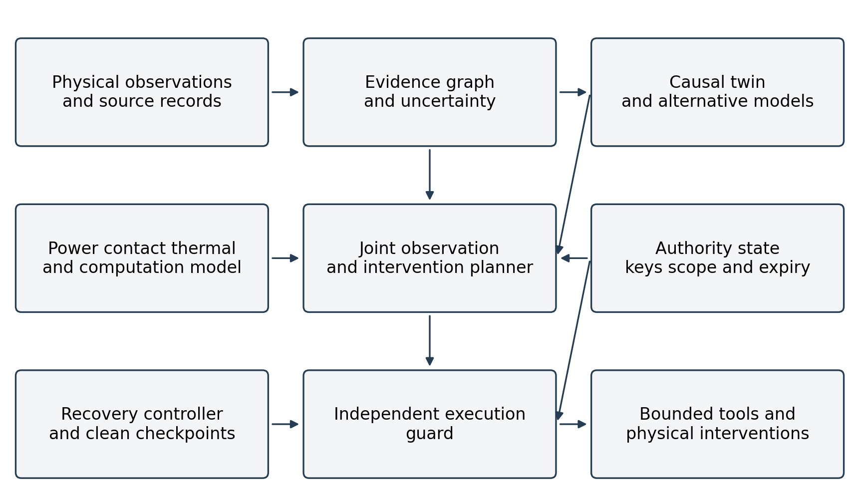
Figure 1 Coupled decision representations and bounded execution. Independent observation of external effects returns through the evidence process.
This division permits different implementation methods. The causal model may combine physical equations with statistical estimates. The planner may use finite search, optimisation or learned proposals. The guard may use deterministic rules and verified components. The scientific requirement is that the interfaces preserve the conditions under which each output is valid. A natural-language summary can accompany the interfaces but cannot replace their machine-checkable fields.
Table 2 Interface records required for a controllable decision
| Interface | Minimum record | Acceptance question |
|---|---|---|
| Observation to evidence | Source acquisition time frame calibration and digest | What was physically measured and under which conditions |
| Evidence to twin | Ancestry uncertainty alternatives and invalidation state | Which state or effect claim does this evidence support |
| Twin to planner | Intervention effect bounds target and transport assumptions | Will the candidate action improve the defined outcome |
| Resources to planner | Completion time energy temperature memory and continuation | Can the information arrive and the system remain recoverable |
| Planner to guard | Target operation parameters delegation expiry and evidence version | Is this exact external effect currently admissible |
| Effect to verifier | Independent state observation and completion criterion | Did the intended outcome occur |
| Recovery to operation | Clean state valid keys current policy and residual dependencies | Can service resume without restoring the fault |
Infrastructure restoration
Suppose an observation suggests reduced activity around a substation serving a port. The twin retains several explanations: physical damage, planned maintenance, upstream load reduction and sensor error. A broad image provides spatial context, but a local diagnostic may more directly distinguish an electrical fault from planned operation. The planner evaluates the expected intervention value of each observation at its delivery time, taking account of an available communications window and the permitted restoration deadline.
If a diagnostic supports a bounded protective reduction, the planner can propose that action under a defined parameter range and expiry. The guard checks the actual target, authority and evidence version before execution. A separate measurement verifies the resulting electrical state. If the expected effect is absent, the system does not mark the mission complete merely because the command was accepted. It revises the hypothesis and follows an authorised recovery or investigation path.
The industrial model can change the objective. Restoring the substation may not restore port throughput if a specialised component supplier remains unavailable. Conversely, preserving a smaller electrical load may support a critical production line while broader repair continues. The action must therefore be assessed through the causal dependency chain, including competing demands and the time required for production to resume.
Space supported logistics and navigation
For a time-sensitive logistics decision, compact onboard processing may deliver a useful indication before a raw-data transfer can complete. A later contact sequence may reverse that preference by allowing high-quality raw data to reach ground processing quickly. The architecture selects between these options using the same decision objective and explicit resource trajectory. It does not assume that processing in space is always preferable or that ground processing is always available.
Navigation integrity connects directly to evidence quality. A well-classified image associated with the wrong location can direct an intervention to the wrong asset. The evidence record must carry registration uncertainty and the navigation solution on which it depends. Specialised inertial or gravity measurements become relevant when they resolve an uncertainty that affects the intervention. Their value is assessed against the actual geometry and deadline, not a generic claim of navigation independence.
Cyber diagnosis and controlled repair
An authorised cyber task begins with a scoped observation, such as reading specified logs or configuration state. An assessment agent identifies competing explanations and may request an additional diagnostic. A repair agent constructs a candidate in isolation. Independent checks evaluate its effect and compatibility. The planner then considers deployment timing, service consequences and recovery resources.
A high-confidence repair without deployment authority remains a proposal. A validly authorised repair that would interrupt critical service at the wrong time may be deferred. An action within its permission scope can still be causally harmful, so the causal and physical evaluations remain necessary after access control succeeds. The guard bounds what can happen; the decision process must still justify why the permitted action should happen.
14 Reproducible computational study
Purpose and experimental catalogue
We implement a finite decision problem to test whether joint sensing and computation placement can change a feasible intervention policy. The study contains four observation modes, a binary hazard, a two-observation depth limit, a discrete schedule and continuous energy and temperature states integrated within each schedule interval. Every observation branch is enumerated. The computation is therefore exact within the declared action catalogue and numerical physical model; it is not an approximation to an unrestricted policy search.
The prior hazard probability is 0.10. An intervention costs three utility units regardless of whether a hazard is present. If the hazard is present, avoided loss is 30 multiplied by one minus the completion slot divided by sixteen. The declining benefit represents a narrowing intervention opportunity. A policy can abstain with zero intervention value. Observation costs are charged whether the result is positive or negative.
Table 3 Assumed observation modes in the finite experiment
| Mode | Sensitivity | False positive | Cost | Delivery and availability |
|---|---|---|---|---|
| Telemetry | 0.75 | 0.040 | 0.15 | One slot; terrestrial feed required |
| Cyber audit | 0.65 | 0.015 | 0.20 | Two slots; terrestrial feed required |
| Orbital compact | 0.86 | 0.050 | 0.20 | Acquire process then one contact slot |
| Orbital raw | 0.97 | 0.020 | 0.25 | Acquire two contact slots then ground processing |
Observation likelihoods are assumed and conditionally independent across the three evidence roots given the binary hazard. Compact and raw orbital observations share an optical root and cannot both be counted as separate observations within one policy. This prevents a policy from receiving duplicated credit for two processing paths from the same source. More complicated dependence would require a joint likelihood model rather than the product used here.
The horizon contains twelve five-minute slots. An eighteen-slot orbital cycle has twelve illuminated slots and six eclipse slots. Solar generation is 32 W in illumination; bus load is 14 W throughout. Battery capacity is 40 Wh, reserve is 3 Wh, and charging and discharging efficiencies are both 0.9. The initial energy is either 12 or 24 Wh. The initial temperature is either 305 or 329 K, thermal capacitance is 1,800 J/K, effective emissivity-area is 0.04 m², and the maximum temperature is 330 K. An additional external heat input of 6 W applies in illumination.
Contact opportunities occur at orbital phases 2, 6, 7, 12, 13 and 14. An optical acquisition occupies one slot with 8 W additional load. Compact processing occupies one slot with 28 W additional load, followed by one contact slot with 25 W additional transmission load. Raw transfer needs two contact slots at that transmission load, followed by one ground-processing slot. Terrestrial telemetry needs one slot and a cyber audit two slots, with no additional orbital load beyond the bus.
Ground electrical demand is outside this deliberately small physical model. The ground-processing slot represents delivery latency rather than a complete ground resource budget. This omission prevents interpreting the raw-versus-compact comparison as a measured total energy advantage. A complete system evaluation must include the omitted ground resources, queue and service availability.
Policy definitions and feasibility
The joint policy can acquire up to two distinct evidence roots and choose a wait of zero to three slots before each acquisition. Transmission then uses the earliest available contacts. Every candidate must complete before the authority expiry and the twelve-slot horizon. Its energy and temperature trajectory must remain within limits, and it must leave a feasible bus-only hold through the horizon. The policy compares each observation plan with acting immediately or abstaining.
The one-observation policy uses the same catalogue, waits, objective and physical constraints but can acquire only one observation. The information-greedy policy chooses the feasible observation with the largest expected entropy reduction per unit observation cost, breaking a tie in favour of earlier completion. It can then make one further greedy acquisition from a distinct root. It is allowed to stop when its selected acquisition would have lower value than acting or abstaining. This avoids constructing an artificially weak comparator that must buy information it cannot use.
The regime grid contains three initial orbital phases, two initial energies, two initial temperatures, two terrestrial-feed states and two authority expiries, giving 48 equally weighted configurations. The initial phases are 0, 8 and 12; authority expires at slot 6 or slot 12. Equal weighting is a design choice for exposing conditions, not an estimate of how often those conditions occur operationally.
Aggregate policy results
Table 4 Means across 48 equally weighted configurations
| Metric | Joint | One observation | Information greedy |
|---|---|---|---|
| Net utility | 1.17949 | 1.11416 | 1.03837 |
| Expected avoided loss | 1.68969 | 1.49164 | 1.53423 |
| Expected intervention cost | 0.29838 | 0.25456 | 0.28832 |
| Expected observation cost | 0.21182 | 0.12292 | 0.20753 |
| Probability of intervention | 0.09946 | 0.08485 | 0.09611 |
| Probability of false intervention | 0.03367 | 0.02719 | 0.02778 |
| Terminal decision time minutes | 12.0492 | 7.6042 | 17.8825 |
The joint policy has strictly greater net utility than the one-observation policy in 24 configurations and than the information-greedy policy in 16. Because its search space includes the feasible alternatives used by the one-observation comparator, non-inferiority is partly a structural property of the experiment. The numerical differences establish how much the added conditional observation and placement choices are worth under these parameters.
The advantage is not free. The joint policy incurs more observation cost than the one-observation policy and acts more often when no hazard is present. Its probability of a false-positive intervention is 0.03367, compared with 0.02719 for one observation and 0.02778 for the information-greedy policy. The common intervention cost in the model penalises these actions, but a mission with greater false-action harm could prefer a different policy. A claim of superiority that omitted this trade-off would overstate the result.
The reported mean terminal decision time includes abstention branches. It is not the mean delay conditional on an intervention. The joint policy terminates in about 12.05 minutes on average, one observation in 7.60 minutes and the information-greedy policy in 17.88 minutes. Earlier termination alone does not determine utility because a second observation can justify an action that a faster policy would miss.
Six explanatory configurations
Table 5 Configurations explaining changes in the selected policy
| Case | Initial conditions | Joint first choice | Net utility |
|---|---|---|---|
| A | Phase 0; 24 Wh; 305 K; feeds; expiry 12 | Telemetry | 1.75704 |
| B | Phase 0; 24 Wh; 305 K; no feeds; expiry 12 | Orbital compact | 1.50325 |
| C | Phase 0; 24 Wh; 329 K; no feeds; expiry 12 | Abstain | 0 |
| D | Phase 12; 12 Wh; 305 K; no feeds; expiry 12 | Abstain | 0 |
| E | Phase 8; 24 Wh; 305 K; no feeds; expiry 6 | Orbital compact | 1.18075 |
| F | Phase 12; 24 Wh; 305 K; no feeds; expiry 12 | Orbital raw | 1.58750 |
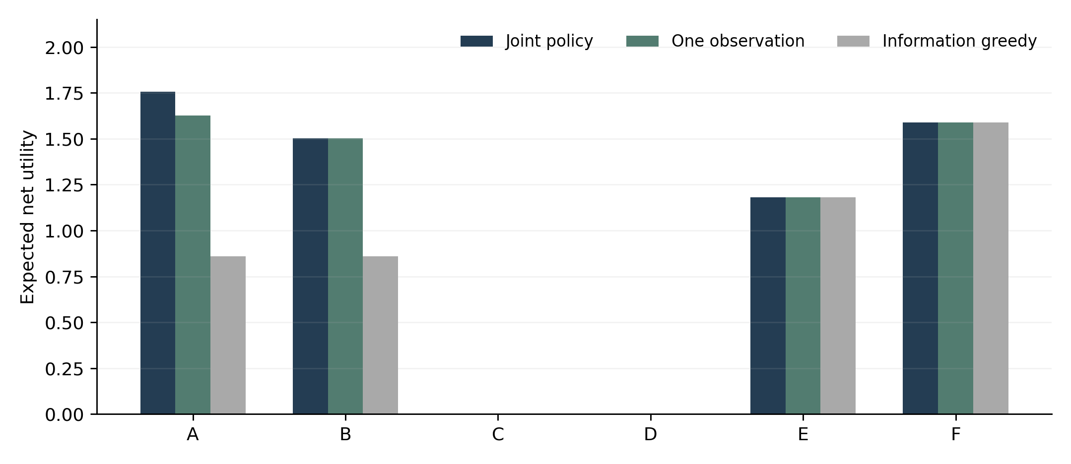
Figure 2 Expected net utility in six configurations. The policies share the same objective feasible observations and physical constraints.
In case A, terrestrial telemetry is acquired first. A positive result is sufficient to justify intervention. A negative result leads to a cyber audit, whose positive result can still justify action before benefit declines too far. This conditional sequence has utility 1.7570. The one-observation policy uses telemetry alone, with utility 1.6264. The information-greedy policy initially favours the higher-quality raw orbital observation, but its delivery is late enough to reduce utility to 0.8600.
In case B, terrestrial feeds are absent. Compact orbital processing completes at slot 3 and yields utility 1.5033, while raw processing completes at slot 8 and yields 0.8600. In case F, the contact geometry changes: raw processing completes at slot 4 and becomes the preferred choice, with utility 1.5875. These cases establish that the same observation-quality ordering can imply different placement decisions once delivery time is included.
Cases C and D make the constraints active. A hot initial state prevents a useful orbital workload in C, while the low-energy eclipse condition in D prevents the required feasible continuation. All three policies abstain. Case E permits compact processing before a short authority expiry and yields utility 1.1808. The model therefore produces a mixture of useful action, conditional investigation and constrained abstention rather than forcing activity in every configuration.
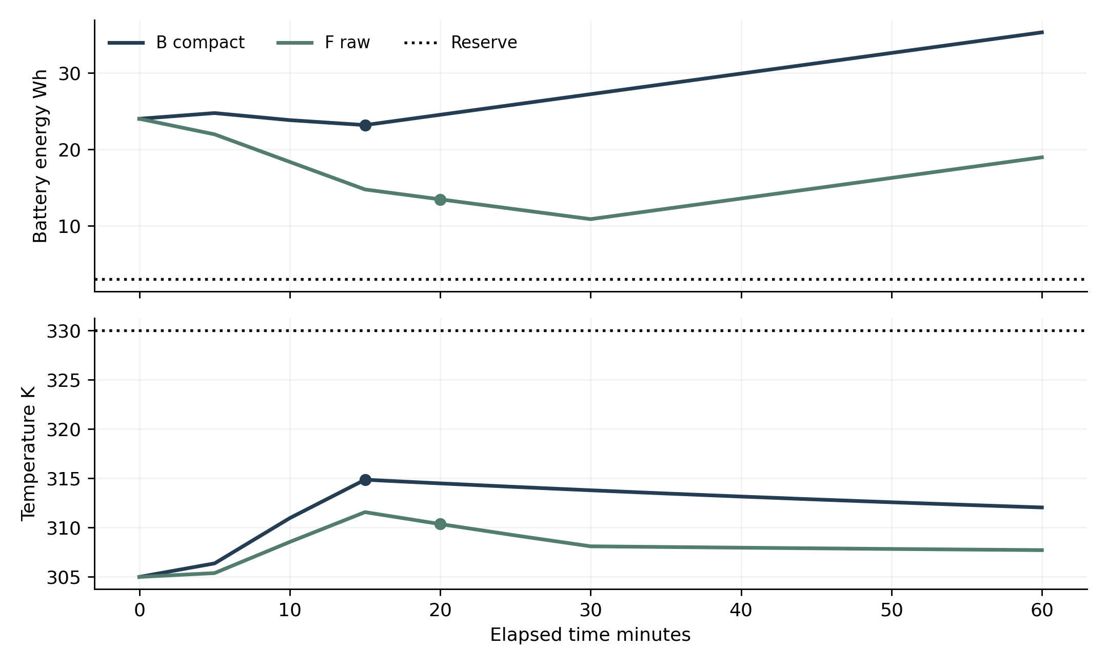
Figure 3 Job and continuation trajectories for compact processing in case B and raw processing in case F. Dots mark observation completion.
The resource trajectories show why post-completion feasibility matters. Energy and temperature continue to evolve after the observation arrives. A job that finishes above the reserve can still be unacceptable if the remaining eclipse drives energy below the required floor. Conversely, a feasible low-temperature trajectory may permit a burst of processing that an average-load rule would reject. These are model-based scheduling effects that require hardware validation before operational use.
Evidence industrial and rare-event exercises
The duplicated-likelihood exercise reproduces the posterior inflation described in Chapter 6. The correlated-estimate exercise evaluates the actual exceedance of a nominal 99% bound when ten Gaussian assessment errors have common pairwise correlation. At correlations 0, 0.2, 0.5, 0.8 and 1, the exceedance probabilities are approximately 1.00%, 12.37%, 27.21%, 36.84% and 41.53%. The calculation makes the confidence consequence of ignored dependence explicit.
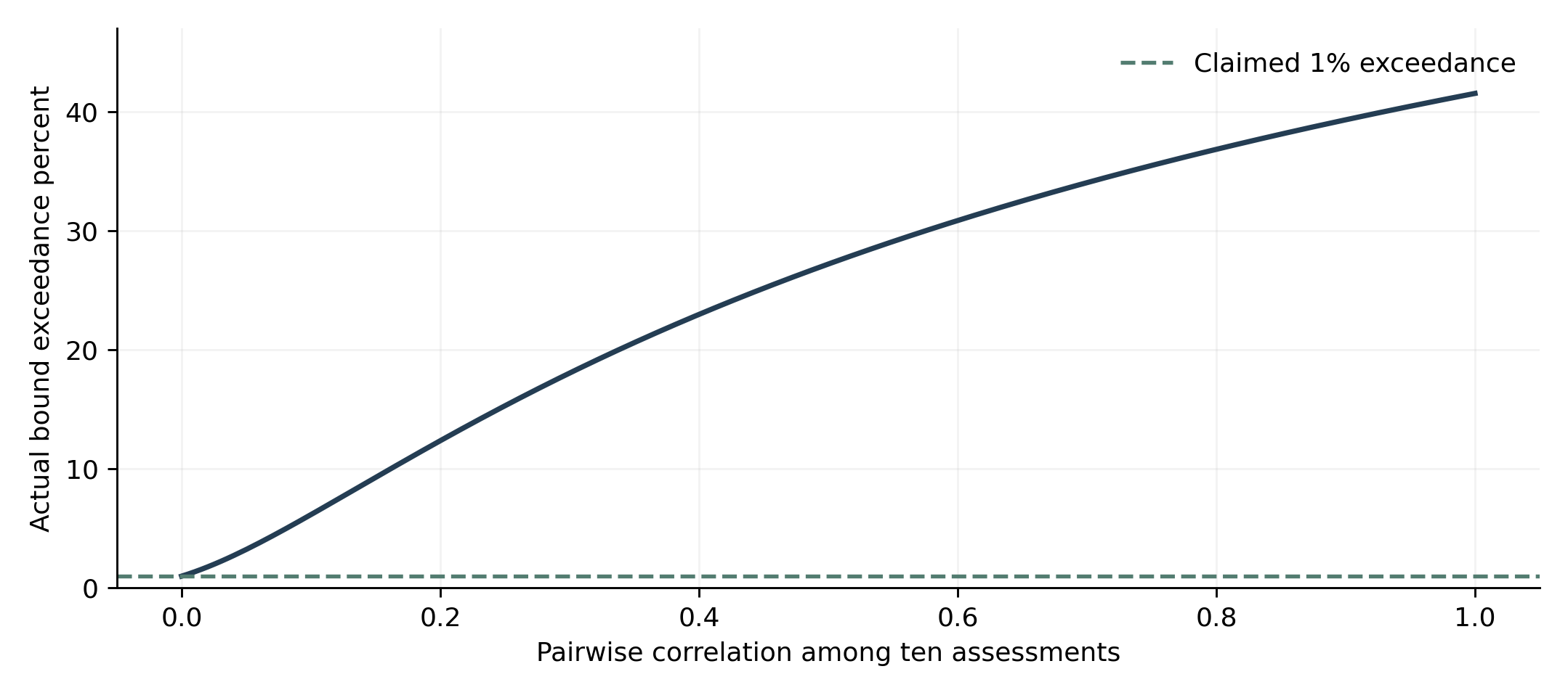
Figure 4 Actual exceedance of a nominal 99% Gaussian bound when ten equally precise estimates share pairwise correlation ignored by the bound.
The industrial exercise uses daily inventory conservation. Deliveries arrive, each manufacturer produces up to ten components using its available input, and final assembly consumes one of each component up to ten units per day. Under concentration, final output is two units on the first day and zero thereafter. Under diversification, it is seven units on the first day and five on each following day. Delayed substitution gives two, zero, five and five units. Larger opening inventories under concentration give ten units on the first day and none thereafter.
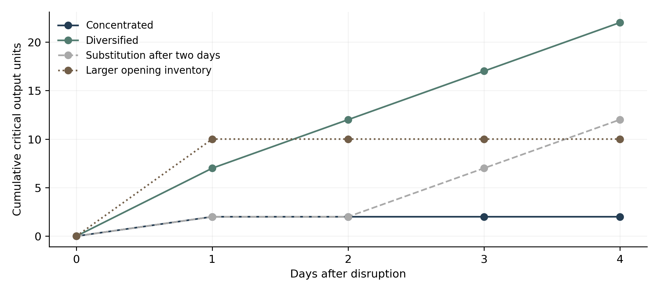
Figure 5 Cumulative critical output under the specified four-day disruption. Initial inventories qualification delay and topology change the consequence.
The conformal interval exercise uses NumPy’s default random generator with seed 7,182,018. It sorts 2,000 absolute standard-normal calibration residuals and selects rank 1,901, corresponding to the finite-sample 95% construction. The resulting half-width is 1.952974. A single vector of 200,000 standard-normal draws supplies both the nominal residuals and the shifted residuals obtained by multiplying by two and adding one. Using paired draws makes the distribution change reproducible.
Nominal coverage is 189,988 out of 200,000, or 94.994%, with a two-sided exact 95% binomial interval of approximately 94.898% to 95.089%. Shifted coverage is 122,866 out of 200,000, or 61.433%, with interval 61.219% to 61.646%. These intervals describe Monte Carlo sampling uncertainty for the fixed calibrated interval and the specified independent test draws. They do not bound performance under an unspecified real-world shift.
The authority exercise evaluates five command records against a fixed contract. One correctly scoped read of asset A, before expiry and under the current policy epoch, is admitted. A write, a read of another asset, a late read and a read under an obsolete epoch are rejected. This checks the contract logic. It is not a penetration test of a deployed authorisation system and does not establish the absence of bypass paths.
Verification and interpretation
The computation checks all 290 terminal policy leaves for branch-probability conservation, feasible continuation and valid intervention timing. Posterior probabilities satisfy the prior martingale identity when averaged over the observation branches. The reported utility equals expected avoided loss minus intervention and observation costs. Inventory quantities remain non-negative and production respects the specified recipe and capacity.
The physical integration uses 60-second substeps within each five-minute slot. Repeating the joint-policy calculation with 30-second and 10-second substeps leaves all 48 initial choices and expected utility values unchanged. This is a numerical sensitivity check for the selected regime grid, not proof of accuracy for every possible initial state. Thermal or energy conditions close to a constraint boundary require finer analysis and hardware comparison.
The nominal and shifted coverage fractions are also checked against their exact Gaussian probabilities for the realised interval width. Both fall within four binomial standard errors. The causal counts reproduce the reported observed and interventional differences, and the industrial totals reproduce the daily conservation calculation. These checks establish internal consistency of the exercises. They leave the principal empirical task intact: measuring the likelihoods, resource dynamics, faults and consequences of an actual operational system.
15 Independent evaluation and architecture review
Evaluation separated from system construction
The validation programme should be administered by a team that does not control the planner’s training data or acceptance oracle. Scenario generation, hidden fault placement and outcome adjudication must be separated from policy development. Otherwise, the system can be optimised to the evaluator’s assumptions while appearing to generalise. Test conditions should be fixed before the final comparison and include regimes in which abstention is correct as well as regimes in which useful action is necessary.
Training and evaluation splits should separate sites, missions, time periods and disruption episodes. All policies should receive the same available information and the same opportunity to recover. Computational budget, observation cost, authority scope and deadline must be recorded. A faster result from a policy that silently omitted verification is not directly comparable with a result whose completion definition includes an independently observed effect.
Causal and evidence challenges
Causal evaluation should introduce historical decisions based on hidden operator information, selective logging and changes in intervention policy. The test asks whether the system recognises non-identification, produces defensible bounds and chooses an appropriate next observation or bounded intervention. Predictive accuracy should be reported separately from the error in estimated intervention value. Where the effect is identified through an experiment, the comparison must preserve the randomisation or other design assumptions.
Evidence trials should include repeated sources presented through different agents, shared calibration faults, incorrect geolocation and generated products that resemble independent observations. The trial should measure harmful confidence inflation, inappropriate action and the time required to invalidate descendants after contamination is discovered. An ablation should disable the actual provenance-dependent decision mechanism rather than merely remove a displayed source label.
The fusion test should distinguish arbitrary outliers from shared honest error. A robust aggregator that succeeds against extreme values can fail against a coherent biased cluster. Fault placement should vary across the communications graph and across evidence roots. Reported robustness must identify the corruption bound, the topology and whether the compromised participants can create additional identities.
Physical and execution trials
Space–ground scheduling requires hardware-in-the-loop tests with measured power and thermal response. Trials should include missed contacts, partial transfers, clock uncertainty, model-version mismatch and interrupted computation. The measurement boundary should include conversion, memory, cryptographic processing and delivery validation. Fault injection should distinguish detected restartable corruption from silent state corruption and persistent hardware faults.
Execution trials should exercise every external-effect path, including queues, retries, scheduled jobs and recovery workers. A command accepted before revocation but executed afterwards is a different case from a command rejected at submission. The evaluator should measure unauthorised effects, harmful authorised effects and beneficial completion separately. Access control can be correct while the planner selects a poor action within its scope.
Recovery tests should remove the primary identity provider, make the most recent checkpoint untrustworthy and interrupt the update path. Success requires restoring defined service without resurrecting obsolete permissions or contaminated evidence. Recovery time should begin at the actual loss of function and end at independently verified service, rather than at process restart. The resources consumed during recovery belong in the mission account.
Industrial and rare-event evaluation
Industrial validation should use independently verified relationships withheld from reconstruction, along with actual input recipes, qualification delays and usable inventories where available. The principal target is the predicted output consequence of disruption and intervention. Graph similarity alone is insufficient because a small error around a bottleneck can dominate the outcome. Testing should also examine actions that redistribute scarce inputs and thereby impose losses elsewhere.
Rare-event evaluation should report lead time, false alerts per operational period, investigation load, missed events, abstentions and the consequences of incorrect action. Confidence intervals should reflect clustering by mission or incident. Thresholds should be fixed before evaluation, and prevalence should be stated. A result obtained on an artificially balanced dataset cannot be interpreted directly as operational precision.
An assurance case that can be invalidated
The assurance case links each claim to assumptions, evidence, responsible components and a condition that would invalidate it. This follows the systems perspective that safety depends on interactions and constraints across the complete operation (Leveson, 2011). A component certificate cannot stand in for the evidence needed at the system boundary.
Model updates, sensor replacement, changed authority semantics and new industrial dependencies can invalidate parts of the case. The system should identify which claims require re-evaluation when those changes occur. Architecture review should ask whether that invalidation actually changes execution. An assurance record that remains green regardless of the operating state has become documentation rather than control.
16 Conditional scenarios through 2040
Mechanisms rather than benchmark extrapolation
We construct scenarios through 2040 around mechanisms that could change the joint decision problem. The scenarios are conditional on measured improvements, deployment constraints and supporting assurance. They do not assume that progress in a model benchmark transfers directly to autonomous operational capability. Their purpose is to identify which evidence would justify a larger action scope or a different distribution of computation.
The principal hypothesis is that observation, computation and intervention become more tightly coupled as systems operate across intermittent networks and constrained platforms. When connectivity and resources are abundant, a simpler centralised design can remain preferable. The importance of joint planning rises when delays, power limits, evidence uncertainty and delegated authority make locally optimal choices conflict.
Table 6 Conditional development scenarios and evidence gates
| Period | Conditional capability | Evidence needed before expanded scope |
|---|---|---|
| Early to mid 2020s | Bounded tool use and independent execution guards | No bypass paths; useful completion; valid recovery under faults |
| Mid 2020s to early 2030s | Multimodal inference and adaptive edge ground orbit placement | Withheld-regime decision value; complete power thermal and delivery measurements |
| 2030s to 2040 | Federated autonomy with specialised sensing and acceleration | Interoperable authority; independent navigation truth; end-to-end efficiency; clean recovery |
Multimodal inference and longer action sequences
Improved multimodal modelling could reduce the effort needed to connect images, sensor histories, documents and operational records. Its value would lie in extracting decision-relevant structure and identifying useful observations. Better synthesis would also make provenance more important because generated products could be mistaken for new measurements. The appropriate evidence gate is improved decision quality under withheld conditions, including cases where modalities share an error.
Longer autonomous action sequences could reduce human coordination burden for bounded tasks. They would also create more opportunities for stale evidence, excessive delegation, retries and cascading effects. Expanded scope should therefore depend on verified state transitions and independently observed completion. Fluent planning or a high task-completion rate under benign conditions would not justify unrestricted tool access.
Containment should evolve with the action catalogue. An agent that only drafts a recommendation has a different consequence profile from one that updates infrastructure state. New capabilities should enter through narrow interfaces whose authority, resource and recovery semantics are explicit. The system can then accumulate evidence for broader use without treating every improvement in language or perception as permission to expand external control.
Specialised sensing and acceleration
Quantum-assisted navigation could become valuable in environments where suitable physical fields and trajectories provide observability and where the sensor can be carried and operated reliably. The condition is stronger than improved instrument sensitivity. The complete estimator must show bounded errors under motion, bias, map uncertainty and denied external positioning, with independent truth for validation.
Photonic and other specialised accelerators could change computation placement when they improve end-to-end performance at the required precision and environmental conditions. A lower arithmetic energy cost is insufficient if conversion, memory, calibration or fault recovery dominates the workload. The relevant milestone is a reproducible improvement in delivered decision value per constrained resource, accompanied by acceptable failure behaviour.
Space computing could expand from selective processing to more complex distributed workloads if power, thermal rejection, communications and recovery mature together. The architecture should not presume continuous cloud-like availability in orbit. Contact geometry and physical survival remain part of the computation contract even when processors become substantially faster.
Demand can exceed efficiency gains
To examine the interaction between workload demand and efficiency, let annual demand growth be d and annual efficiency improvement be e. Holding the simplified relationship constant for 22 years gives the following energy-demand ratio relative to the starting point.

Equation 11 Conditional 2040 energy-demand ratio under constant annual demand and efficiency changes.
With demand growth of 5% and efficiency improvement of 9%, the ratio is approximately 0.439. With demand growth of 10% and efficiency improvement of 6%, it is 2.259. With demand growth of 15% and efficiency improvement of 3%, it is 11.296. These are arithmetic scenarios, not fitted forecasts. They show that improved efficiency can coexist with sharply increasing total energy demand.
The physical implications differ across platforms. A ground installation may expand power and cooling at substantial cost. A spacecraft has strict limits on mass, area, thermal rejection and storage. The planner must therefore manage demand as well as exploit efficiency. It can prioritise decision-relevant computation, defer low-value tasks, choose approximations and avoid redundant processing of dependent evidence.
Federated sovereignty
By 2040, greater federation could increase both useful redundancy and dependence on shared services. Interoperable data formats would not by themselves make causal assumptions, authority semantics or recovery procedures interoperable. One participant’s confidence statement may have different validity conditions from another’s. One participant’s emergency permission may not authorise action on another’s infrastructure.
A credible federation would exchange explicit contracts, evidence ancestry and bounded delegations. It would preserve the ability to contain a compromised participant without collapsing every shared function. The evidence for sovereignty would remain practical: which services continue, which actions stay controlled and how independently the operator can recover. The date does not change that test.
17 Conclusions
The central research question requires a policy over observations, computation and authorised intervention. Optimising any one of these in isolation can produce an accurate but ineffective forecast, a timely but unjustified action, or a useful result that cannot be delivered within physical limits. We have proposed an architecture that retains the causal, evidential, resource and authority conditions needed to connect intelligence to an external effect.
The constructive exercises expose distinct failure mechanisms. Confounding reverses the apparent sign of an intervention effect. Repeated evidence produces extreme confidence without new observation. Identical industrial totals conceal sharply different bottleneck outcomes. A valid nominal prediction interval loses coverage after a specified distribution shift. None of these problems is solved merely by increasing model capacity or the number of agents.
The finite joint-policy experiment shows how contact geometry, thermal state, energy reserve and authority expiry can change the preferred observation and computation path. Under the stated parameters, joint selection improves expected net utility over feasible one-observation and information-greedy alternatives. The increase comes with additional observation cost and more false-positive interventions. Its practical value therefore depends on measuring consequences and calibrating the objective for the intended mission.
Assured autonomy requires enforceable boundaries and a recovery path. Evidence must remain traceable through transformations, permissions must be checked at the external effect, and recovery must restore clean state without reviving obsolete authority. Agreement among agents, a verified component or an efficient accelerator can contribute to that result only under the assumptions that connect it to the complete system.
The next research stage is independent end-to-end evaluation. It must measure causal intervention value, useful completion, harmful action, alert burden, resource trajectories and recovery under conditions the system developers do not control. The appropriate standard is a demonstrated ability to improve outcomes while remaining controllable under declared disruptions. That standard provides a coherent basis for conditional development through 2040.
Appendix A Formal arguments and assumptions
A1 Partial identification of the intervention effect
Let Y(1) and Y(0) be binary potential failure outcomes with and without intervention, and let A be the observed intervention. Consistency identifies Y(1) for treated cases and Y(0) for untreated cases. In the constructed population, Pr(Y = 1, A = 1) is 0.076 and Pr(A = 0) is 0.74. The unobserved treated potential outcomes of untreated cases can range from all zero to all one. Therefore E[Y(1)] lies between 0.076 and 0.816.
Similarly, Pr(Y = 1, A = 0) is 0.088 and Pr(A = 1) is 0.26, giving E[Y(0)] between 0.088 and 0.348. Subtracting the largest feasible untreated mean from the smallest treated mean gives −0.272. Subtracting the smallest untreated mean from the largest treated mean gives 0.728. The endpoints are attainable by suitable assignments of the unobserved binary potential outcomes. No unconfoundedness or monotonicity restriction has been imposed. The bounds therefore describe what the treatment-outcome table alone permits under consistency (Manski, 1990).
A2 Generated representations and conditional information
Assume G = g(Y, θ, R), with R independent of X conditional on Y and θ. For fixed Y and θ, the conditional distribution of G depends on R and the mapping g, not on X. The joint conditional distribution of X and G consequently factors into their conditional marginals. Their conditional mutual information is zero. The conclusion concerns information beyond the measured data and the fixed model, not the computational ease of extracting that information (Cover and Thomas, 2006).
If θ is uncertain and informative about X, conditioning on θ matters. If the generator receives an additional physical observation, that observation belongs in the conditioning set. If the generated output is used as a convenient statistic, it may improve a resource-constrained decision without adding an independent measurement. These distinctions prevent the information statement from being misread as a claim that representation learning has no value.
A3 Conditional preservation of safety and recovery
Let the information state contain the set of physical states consistent with delivered evidence, together with resources, authority and persistent model variables. Define K as a set of information states from which one admissible observation-based policy can maintain the declared constraints and reach an acceptable terminal or recovery condition for every disturbance admitted by the model. The same policy must work across the unresolved states; choosing a different policy with knowledge of the hidden state would not establish recoverability under partial observation.
Assume the initial information state lies in K, every admitted action respects constraints over its full duration, and every possible successor information state remains in K. Also assume that the execution guard is uncompromised, covers every external-effect path, and checks valid, unforgeable authority under the declared commit semantics. Induction over decision steps then preserves membership in K and the corresponding constraints. The base case is the initial condition; the inductive step follows from the admitted-action and successor conditions.
This argument is conditional on model coverage, guard correctness and the semantics of durative actions. It establishes preservation of the specified property, not progress towards every mission goal. It does not cover a physical disturbance excluded from the model or an authority bypass excluded from the implementation assumptions. A useful assurance case identifies evidence for those assumptions and the operational response when they fail.
A4 Revocation during disconnection
Construct two global histories whose local projection at the executor is identical. In one history the issuer revokes a grant after disconnection; in the other it does not. Any deterministic executor rule based only on the local projection selects the same action in both histories. A randomised rule likewise has the same action distribution in both. Immediate enforcement of the unseen revocation together with unrestricted continuation in the unrevoked history is therefore impossible without an additional information or authority assumption.
Leases, trusted time bounds and explicitly delegated local emergency powers alter the contract and can bound consequences. They do not refute the indistinguishability argument. A correct design states those mechanisms as part of the authority semantics rather than claiming immediate global knowledge during a partition.
Appendix B Computational specification and reproduction
B1 Finite policy recursion
At each information state, the computation first evaluates immediate intervention and abstention. If observation depth remains, it enumerates each unused evidence root, its permitted processing mode and waits from zero to three slots. It propagates the energy and thermal state through acquisition, processing and communications, checks delivery and authority timing, and tests the required continuation. Infeasible candidates are removed.
For each feasible observation, Bayes’ rule gives positive and negative branch probabilities and posteriors. The recursion evaluates each successor policy, takes their probability-weighted value and subtracts observation cost. The largest value, including immediate termination, is retained. The one-observation comparator changes the maximum depth to one. The information-greedy comparator restricts each acquisition choice to the feasible observation with the greatest entropy reduction per cost before evaluating whether to continue.
VALUE(history, state, depth)
best = max(value_of_permitted_action, 0)
if depth == 0: return best
for each feasible unused observation and wait:
next_state = propagate_resources_and_delivery()
if continuation_or_authority_invalid: continue
value = -observation_cost
for each result and Bayesian posterior:
value += probability * VALUE(updated_history,
next_state, depth - 1)
best = max(best, value)
return best
The search does not include arbitrary concurrent workloads, unlimited waiting, repeated optical roots or more than two observations. These restrictions define the finite claim. A larger planner would need additional algorithms and validation, including treatment of the physical state during concurrent processing and communications.
B2 Numerical and statistical settings
The physical model uses forward time integration with 60-second increments, repeated at 30 and 10 seconds for sensitivity. Battery charging is curtailed at 40 Wh, while reserve and thermal constraints are checked after each increment. The radiation discussion is an analytical checkpoint example and is not part of the finite scheduling simulation. There is no simulated empirical radiation-rate estimate.
The coverage exercise uses seed 7,182,018, 2,000 calibration draws and 200,000 paired test draws. The exact Gaussian coverage for the realised interval half-width is computed separately from the Monte Carlo fraction. The binomial intervals describe the independent test-sample uncertainty conditional on that half-width. Repeating the whole calibration procedure would introduce another source of variation requiring a separate analysis.
The industrial exercise has two component manufacturers and one final-assembly requirement using one unit of each component. Daily deliveries precede production, and components can be carried between days. Substitution after two days changes the delivery allocation from day three. Units are abstract compatible production units, so the example does not claim a particular industry’s throughput or substitution time.
B3 Reproduction and sensitivity priorities
An independent reproduction should first recover the causal counts, policy branch probabilities, utility decomposition and inventory totals. It should then reproduce the 48 regime results, the six explanatory cases and the coverage fractions. Changing integration resolution tests numerical sensitivity; changing observation likelihoods, consequence weights and physical parameters tests model sensitivity. These are different exercises and should be reported separately.
The highest-priority extensions are explicit false-intervention harm, uncertain observation likelihoods, shared cross-source errors, ground-resource constraints and concurrent jobs. Each extension can change the optimal policy. The correct comparison retains the same extended model and feasible opportunities for every baseline. The model should not be enlarged only for the proposed method while keeping the alternatives artificially restricted.
Appendix C Claim and challenge register
The register summarises the main architecture claims, a condition that could defeat each claim and the evidence needed to assess it. It is intended to guide independent review and subsequent experiments. Passing one challenge does not validate every other row because the assumptions and failure mechanisms differ.
Table 7 Claims challenges and required evidence
| Claim | Defeating condition | Required evidence |
|---|---|---|
| Intervention improves outcome | Historical operators used unrecorded risk information | Identification argument experiment or defensible effect bounds |
| Observation has operational value | Useful result arrives after action deadline | Delivered history and measured completion time |
| Many agents corroborate a claim | Agents repeat one source or one model error | Ancestry and cross-source dependence analysis |
| Generated modality fills a gap | Output reflects a prior rather than a new observation | Trace to actual measurements and withheld truth |
| Orbital computation is feasible | Hot start eclipse missed contact or depleted reserve | Complete measured resource trajectory and continuation |
| Agent faults are contained | Fault placement violates the assumed graph bound | Topology-specific fault trials and scope enforcement |
| Execution is sovereign | Identity update key or recovery dependency disappears | Dependency-removal exercises over the declared duration |
| Industrial disruption is bounded | A compatible hidden network contains a bottleneck | Held-out relationships inventories and output consequences |
| Forecast uncertainty is calibrated | Operating distribution or decision policy changes | Regime-specific coverage and shift response |
| A task is complete | Command acknowledged but physical effect absent | Independent state verification |
| Acceleration saves system resources | Conversion memory and calibration dominate | End-to-end latency energy precision and fault measurements |
| Recovery restores control | Checkpoint revives contaminated data or expired grants | Clean replay current authority and observed restored service |
References
Acemoglu, D., Carvalho, V.M., Ozdaglar, A. and Tahbaz-Salehi, A. (2012) ‘The network origins of aggregate fluctuations’, Econometrica, 80(5), pp. 1977–2016. https://doi.org/10.3982/ECTA9623
Alshiekh, M., Bloem, R., Ehlers, R., Könighofer, B., Niekum, S. and Topcu, U. (2017) ‘Safe reinforcement learning via shielding’, arXiv:1708.08611v1, 29 August. https://arxiv.org/abs/1708.08611v1
Ames, A.D., Xu, X., Grizzle, J.W. and Tabuada, P. (2017) ‘Control barrier function based quadratic programs for safety critical systems’, IEEE Transactions on Automatic Control, 62(8), pp. 3861–3876. https://doi.org/10.1109/TAC.2016.2638961
Bareinboim, E. and Pearl, J. (2016) ‘Causal inference and the data-fusion problem’, Proceedings of the National Academy of Sciences, 113(27), pp. 7345–7352. https://doi.org/10.1073/pnas.1510507113
Barrot, J.-N. and Sauvagnat, J. (2016) ‘Input specificity and the propagation of idiosyncratic shocks in production networks’, Quarterly Journal of Economics, 131(3), pp. 1543–1592. https://doi.org/10.1093/qje/qjw018
Castro, M. and Liskov, B. (1999) ‘Practical Byzantine fault tolerance’, Proceedings of the Third Symposium on Operating Systems Design and Implementation. Berkeley, CA: USENIX. https://www.usenix.org/conference/osdi-99/practical-byzantine-fault-tolerance
Cerf, V., Burleigh, S., Hooke, A., Torgerson, L., Durst, R., Scott, K., Fall, K. and Weiss, H. (2007) Delay-Tolerant Networking Architecture. RFC 4838. Internet Research Task Force. https://doi.org/10.17487/RFC4838
Clopper, C.J. and Pearson, E.S. (1934) ‘The use of confidence or fiducial limits illustrated in the case of the binomial’, Biometrika, 26(4), pp. 404–413. https://doi.org/10.1093/biomet/26.4.404
Cover, T.M. and Thomas, J.A. (2006) Elements of Information Theory. 2nd edn. Hoboken, NJ: Wiley. https://doi.org/10.1002/047174882X
Daly, J.T. (2006) ‘A higher order estimate of the optimum checkpoint interval for restart dumps’, Future Generation Computer Systems, 22(3), pp. 303–312. https://doi.org/10.1016/j.future.2004.11.016
Fawzi, H., Tabuada, P. and Diggavi, S. (2014) ‘Secure estimation and control for cyber-physical systems under adversarial attacks’, IEEE Transactions on Automatic Control, 59(6), pp. 1454–1467. https://doi.org/10.1109/TAC.2014.2303233
Gandy, A. and Veraart, L.A.M. (2017) ‘A Bayesian methodology for systemic risk assessment in financial networks’, Management Science, 63(12), pp. 4428–4446. https://doi.org/10.1287/mnsc.2016.2546
Geiger, R. et al. (2011) ‘Detecting inertial effects with airborne matter-wave interferometry’, Nature Communications, 2, article 474. https://doi.org/10.1038/ncomms1479
Gilbert, S. and Lynch, N. (2002) ‘Brewer’s conjecture and the feasibility of consistent, available, partition-tolerant web services’, ACM SIGACT News, 33(2), pp. 51–59. https://doi.org/10.1145/564585.564601
Gilmore, D.G. (ed.) (2002) Spacecraft Thermal Control Handbook. Volume I: Fundamental Technologies. 2nd edn. Reston, VA: American Institute of Aeronautics and Astronautics. https://doi.org/10.2514/4.989117
Glaessgen, E.H. and Stargel, D.S. (2012) ‘The digital twin paradigm for future NASA and U.S. Air Force vehicles’, 53rd AIAA/ASME/ASCE/AHS/ASC Structures, Structural Dynamics and Materials Conference, AIAA 2012-1818. https://ntrs.nasa.gov/citations/20120008178
Gneiting, T. and Raftery, A.E. (2007) ‘Strictly proper scoring rules, prediction, and estimation’, Journal of the American Statistical Association, 102(477), pp. 359–378. https://doi.org/10.1198/016214506000001437
Golovin, D. and Krause, A. (2011) ‘Adaptive submodularity: Theory and applications in active learning and stochastic optimization’, Journal of Artificial Intelligence Research, 42, pp. 427–486. https://doi.org/10.1613/jair.3278
Goodfellow, I.J., Pouget-Abadie, J., Mirza, M., Xu, B., Warde-Farley, D., Ozair, S., Courville, A. and Bengio, Y. (2014) ‘Generative adversarial nets’, Advances in Neural Information Processing Systems, 27. https://papers.nips.cc/paper/2014/hash/f033ed80deb0234979a61f95710dbe25-Abstract.html
Hollinger, G.A. and Sukhatme, G.S. (2014) ‘Sampling-based robotic information gathering algorithms’, International Journal of Robotics Research, 33(9), pp. 1271–1287. https://doi.org/10.1177/0278364914533443
Horowitz, M. (2014) ‘Computing’s energy problem (and what we can do about it)’, IEEE International Solid-State Circuits Conference Digest of Technical Papers, pp. 10–14. https://doi.org/10.1109/ISSCC.2014.6757323
Hu, V.C., Ferraiolo, D., Kuhn, R., Schnitzer, A., Sandlin, K., Miller, R. and Scarfone, K. (2014) Guide to Attribute Based Access Control (ABAC) Definition and Considerations. NIST Special Publication 800-162, original January edition. Gaithersburg, MD: National Institute of Standards and Technology. https://csrc.nist.gov/pubs/sp/800/162/final
Iyengar, G.N. (2005) ‘Robust dynamic programming’, Mathematics of Operations Research, 30(2), pp. 257–280. https://doi.org/10.1287/moor.1040.0129
Jiang, N. and Li, L. (2016) ‘Doubly robust off-policy value evaluation for reinforcement learning’, Proceedings of Machine Learning Research, 48, pp. 652–661. https://proceedings.mlr.press/v48/jiang16.html
Jouppi, N.P. et al. (2017) ‘In-datacenter performance analysis of a tensor processing unit’, ACM SIGARCH Computer Architecture News, 45(2), pp. 1–12. https://doi.org/10.1145/3140659.3080246
Julier, S.J. and Uhlmann, J.K. (1997) ‘A non-divergent estimation algorithm in the presence of unknown correlations’, Proceedings of the American Control Conference, 4, pp. 2369–2373. https://doi.org/10.1109/ACC.1997.609105
Kaelbling, L.P., Littman, M.L. and Cassandra, A.R. (1998) ‘Planning and acting in partially observable stochastic domains’, Artificial Intelligence, 101(1–2), pp. 99–134. https://www.cassandra.org/arc/papers/aij98.pdf
Klein, G. et al. (2009) ‘seL4: Formal verification of an OS kernel’, Proceedings of the 22nd ACM Symposium on Operating Systems Principles, pp. 207–220. https://doi.org/10.1145/1629575.1629596
Krause, A., Singh, A. and Guestrin, C. (2008) ‘Near-optimal sensor placements in Gaussian processes: Theory, efficient algorithms and empirical studies’, Journal of Machine Learning Research, 9, pp. 235–284. https://www.jmlr.org/papers/v9/krause08a.html
Lamport, L., Shostak, R. and Pease, M. (1982) ‘The Byzantine generals problem’, ACM Transactions on Programming Languages and Systems, 4(3), pp. 382–401. https://lamport.azurewebsites.net/pubs/byz.pdf
LeBlanc, H.J., Zhang, H., Koutsoukos, X. and Sundaram, S. (2013) ‘Resilient asymptotic consensus in robust networks’, IEEE Journal on Selected Areas in Communications, 31(4), pp. 766–781. https://cs.vuse.vanderbilt.edu/koutsoxd/www/Publications/resilientConsensusJSAC2013.pdf
Le Goues, C., Nguyen, T., Forrest, S. and Weimer, W. (2012) ‘GenProg: A generic method for automatic software repair’, IEEE Transactions on Software Engineering, 38(1), pp. 54–72. https://doi.org/10.1109/TSE.2011.104
Leveson, N.G. (2011) Engineering a Safer World: Systems Thinking Applied to Safety. Cambridge, MA: MIT Press.
Manski, C.F. (1990) ‘Nonparametric bounds on treatment effects’, American Economic Review, 80(2), pp. 319–323. https://ipcid.org/evaluation/outros_temas/Manski%20-%20Nonparametric%20Bounds.pdf
NASA (2015) Small Spacecraft Technology State of the Art. NASA/TP–2015–216648/REV1. Moffett Field, CA: Ames Mission Design Division, December. https://www.nasa.gov/wp-content/uploads/2017/03/small_spacecraft_technology_state_of_the_art_2015_tagged.pdf
Page, E.S. (1954) ‘Continuous inspection schemes’, Biometrika, 41(1–2), pp. 100–115. https://doi.org/10.1093/biomet/41.1-2.100
Pearl, J. (2009) Causality: Models, Reasoning, and Inference. 2nd edn. Cambridge: Cambridge University Press.
Peters, J., Bühlmann, P. and Meinshausen, N. (2016) ‘Causal inference by using invariant prediction: Identification and confidence intervals’, Journal of the Royal Statistical Society, Series B, 78(5), pp. 947–1012. https://doi.org/10.1111/rssb.12167
Pohl, C. and van Genderen, J.L. (1998) ‘Multisensor image fusion in remote sensing: Concepts, methods and applications’, International Journal of Remote Sensing, 19(5), pp. 823–854. https://doi.org/10.1080/014311698215748
Robins, J. (1986) ‘A new approach to causal inference in mortality studies with a sustained exposure period—application to control of the healthy worker survivor effect’, Mathematical Modelling, 7(9–12), pp. 1393–1512. https://doi.org/10.1016/0270-0255(86)90088-6
Saito, T. and Rehmsmeier, M. (2015) ‘The precision-recall plot is more informative than the ROC plot when evaluating binary classifiers on imbalanced datasets’, PLOS ONE, 10(3), e0118432. https://doi.org/10.1371/journal.pone.0118432
Saltzer, J.H. and Schroeder, M.D. (1975) ‘The protection of information in computer systems’, Proceedings of the IEEE, 63(9), pp. 1278–1308. https://doi.org/10.1109/PROC.1975.9939
Samuel, J., Mathewson, N., Cappos, J. and Dingledine, R. (2010) ‘Survivable key compromise in software update systems’, Proceedings of the 17th ACM Conference on Computer and Communications Security, pp. 61–72. https://justinsamuel.com/papers/survivable-key-compromise-ccs2010.pdf
Shafer, G. and Vovk, V. (2008) ‘A tutorial on conformal prediction’, Journal of Machine Learning Research, 9, pp. 371–421. https://jmlr.org/papers/volume9/shafer08a/shafer08a.pdf
Shen, Y. et al. (2017) ‘Deep learning with coherent nanophotonic circuits’, Nature Photonics, 11, pp. 441–446. https://doi.org/10.1038/nphoton.2017.93
Shoshitaishvili, Y. et al. (2016) ‘SoK: (State of) The art of war: Offensive techniques in binary analysis’, Proceedings of the IEEE Symposium on Security and Privacy, pp. 138–157. https://doi.org/10.1109/SP.2016.17
Sinclair, D. and Dyer, J. (2013) ‘Radiation effects and COTS parts in SmallSats’, Proceedings of the 27th AIAA/USU Conference on Small Satellites, SSC13-IV-3. https://digitalcommons.usu.edu/smallsat/2013/all2013/69/
Vaswani, A., Shazeer, N., Parmar, N., Uszkoreit, J., Jones, L., Gomez, A.N., Kaiser, Ł. and Polosukhin, I. (2017) ‘Attention is all you need’, Advances in Neural Information Processing Systems, 30. https://proceedings.neurips.cc/paper/2017/hash/3f5ee243547dee91fbd053c1c4a845aa-Abstract.html