Digital Twins and Predictive Intelligence
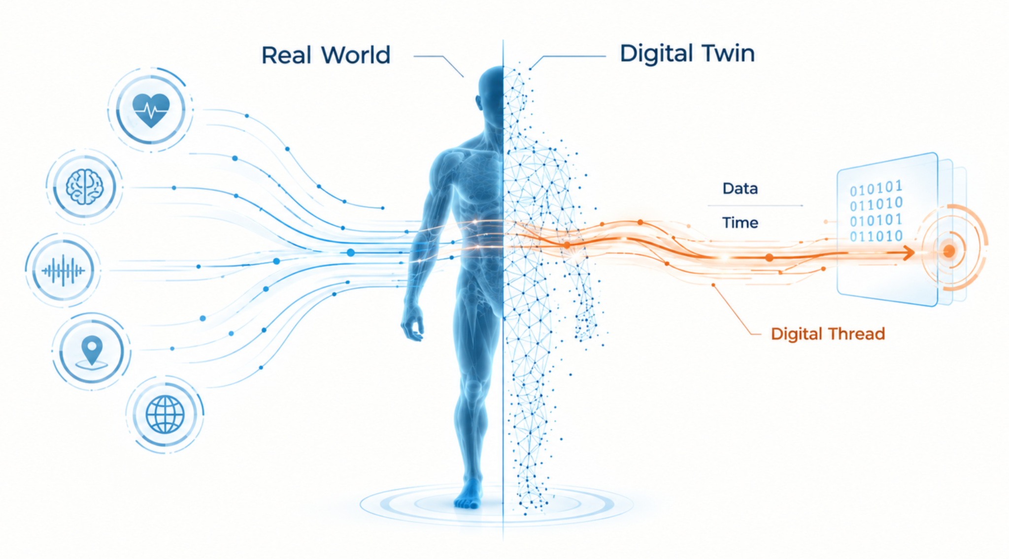
Evidence conditioned architecture for reliable forecasting and operational decisions
Contents
Abstract
Digital twins become useful for predictive intelligence when their representations of physical systems, uncertain observations and feasible interventions remain consistent with one another. A detailed model can nevertheless generate misleading confidence if it treats dependent sources as independent, silently replaces observations with generated data, or evaluates forecasts using information that arrived after the decision. We develop an evidence-conditioned architecture that preserves these distinctions while connecting operational models, geospatial observations, cyber-physical monitoring and place-based public-safety analysis.
Our contribution is a research architecture with explicit evidence and decision contracts, analytical results for dependence and observation age, reproducible synthetic incubation experiments, and an evaluation programme tied to operational outcomes. We separate the physical state, the information available about that state, and the authority to intervene. Modality-specific representations support a joint probabilistic model without erasing provenance or turning latent similarity into a causal claim. Satellite reconstruction, geospatial foundation models and physics-informed surrogates are treated as fallible measurement and simulation components.
In 100 independent replications of 2,000 synthetic episodes per condition, four strongly correlated measurements yield only 61.76% coverage for a nominal 90% interval when independence is incorrectly assumed. Modelling the covariance restores coverage to 89.97%, with a paired Brier-score improvement of 0.00751. Propagating observation age similarly maintains approximately 90% coverage as measurements become stale, at the necessary cost of wider intervals. A reporting experiment constructs two distinct public-safety environments with identical observed-count distributions, demonstrating why recorded incidents alone cannot identify underlying need. Exhaustive evaluation of a finite action guard detects all eight deliberately omitted conditions across 640 input assignments.
These results establish component-level properties under stated assumptions. They motivate a development path in which LupoToro's Digital Twins initiative supplies state and consequence models, while its Predictive Intelligence initiative specifies forecast questions, competing explanations and decision relevance. The principal research objective is demonstrable improvement in decisions under uncertainty, supported by traceable evidence and independently testable limits.
1 Research problem and contribution
1.1 The object of prediction
The central question is whether an evolving representation of an operating system can produce a useful warning early enough to change an outcome. We define the object of prediction before selecting the model. A transport interruption, an abnormal equipment state, an energy shortfall and a rise in recorded incidents have different observability, time scales and intervention mechanisms. Combining their data does not remove these differences. A forecast must specify an event, a time horizon, a spatial or organisational boundary, and the procedure by which its outcome will be determined.
Consider an industrial facility whose commitments depend on power, communications, a transport corridor and replacement components. A satellite image may suggest corridor disruption; a maintenance system may indicate low redundancy; telemetry may reveal deteriorating performance. None alone establishes that a delivery will fail. The relevant inference concerns the joint evolution of the dependency network, the reliability and age of its evidence, and the feasible response. A digital twin contributes a state and consequence model. Predictive intelligence contributes a defined question, competing explanations, and an assessment whose correctness can later be measured.
The engineering tradition gives this coupling a substantial foundation. Early aerospace formulations combined structural models, sensor information and maintenance history around a particular asset (Glaessgen and Stargel, 2012). Subsequent work formalised asset-twin interaction as a probabilistic dynamical system (Kapteyn, Pretorius and Willcox, 2021). We extend the research question across heterogeneous operational domains by making the evidence boundary and decision boundary explicit. This is a design synthesis with tested components, rather than a claim that one general model has already mastered every domain.
1.2 Research questions
We investigate four questions. First, how should a twin represent uncertain and dependent observations without confusing the amount of data with the amount of independent evidence? Second, how can spatial, temporal, semantic and physical models interact while retaining their distinct validation requirements? Third, what prevents a predictive or simulated result from becoming an unsupported operational action? Fourth, what experiments would distinguish useful predictive intelligence from retrospective pattern fitting?
These questions imply three levels of assessment. Statistical validity concerns the relationship between predictions and outcomes. Causal validity concerns the consequences of changing an action. Operational validity concerns whether the complete system can improve an authorised decision within its time, resource and safety constraints. Success at one level does not establish success at the others. For example, correctly predicting a region's reported incident count does not show that a proposed intervention will reduce underlying harm.
1.3 Contributions and scope
We specify a federated architecture with typed evidence records, local physical models, uncertainty-preserving fusion, scenario isolation and a guarded action interface. We derive the loss of effective information under correlated sensing and the increase in uncertainty caused by stale observations. We construct an observational-equivalence example for incident reporting, and test a finite authorisation guard by exhaustive enumeration and condition-removal mutation. The accompanying experiment package contains the code, parameters, replication-level outputs and analytical checks needed to reproduce the numerical results.
The study concentrates on infrastructure resilience, maintenance, supply continuity, disaster recovery and governed public-safety planning. Defence relevance follows from the same requirements for readiness, assurance, uncertain sensing and constrained resource allocation. The proposed architecture does not depend on identifying people as future offenders or automatically converting an intelligence assessment into a coercive action. Its public-safety unit of analysis is a place and time interval with an explicit service objective.
The work supports two named LupoToro research programmes: Digital Twins and Predictive Intelligence, the latter located at the strategic-intelligence website address. Their roles are developed in Section 14. Their programme descriptions establish organisational context; the technical arguments and experimental claims stand on the methods and evidence presented here.
2 Research method and critical synthesis
2.1 Evidence selection
We use a structured critical synthesis rather than a pooled meta-analysis. The corpus connects digital-twin foundations, uncertainty and causal inference, geospatial representation learning, cyber-physical assurance and public-safety modelling. Sources were selected for their direct relevance to a stated architectural choice or an identifiable failure mechanism. Primary papers, author-hosted manuscripts, standards and official technical reports take precedence over marketing summaries. Bibliographic details and the public availability of recent versions were checked against publisher or repository records.
The scientific reference set closed in June 2025. Versioned preprints are cited at a version available within that horizon. A year in a title, a patent priority date or a thesis submission date is insufficient by itself to establish that its results were publicly available. Preprints are identified as such. Standards are cited by edition. We use this horizon as a boundary on the scientific evidence, not as a claim about when the present experiments were conducted.
The synthesis is not exhaustive across all relevant disciplines, and it does not estimate a universal effect size for digital twins. Published evaluations differ in assets, labels, access to ground truth, simulation fidelity and decision objectives. Treating their reported accuracies as directly comparable would obscure those differences. Our quantitative claims therefore come from fully specified experiments within this study, while external results motivate components and evaluation choices.
2.2 What qualifies as a twin
The literature does not support equating every three-dimensional representation or dashboard with a digital twin. Kritzinger and colleagues distinguish digital models, digital shadows and twins by their data integration and directional coupling (Kritzinger et al., 2018). Jones and colleagues identify a broader set of characteristics, including physical and virtual entities, environments, state and twinning processes (Jones et al., 2020). These accounts help explain why visual detail alone is an inadequate measure of capability.
We use the term predictive twin for a maintained representation of an identifiable system that incorporates observations, generates testable predictions, and supports a decision-feedback process. The feedback may be mediated by an authorised human. An observation-only deployment is described as a shadow where that distinction matters. Automatic actuation is an additional engineering capability, with its own assurance obligations, rather than a terminological requirement that justifies adding control authority prematurely.
The National Academies' synthesis places mathematical, statistical and computational gaps at the centre of digital-twin development (National Academies, 2024). Modelling surveys also identify the importance of combining data, simulation and application requirements (Rasheed, San and Kvamsdal, 2020). A consequence for this study is that fidelity must be defined relative to a question. A simple model may be sufficient for maintenance scheduling while a high-resolution model remains inadequate for a rapid safety decision. We therefore attach a declared domain of validity, uncertainty description and decision horizon to each model.
2.3 The relevant frontier
Four research strands are particularly relevant. Probabilistic graphical models provide a principled connection between state, observation and control (Kapteyn, Pretorius and Willcox, 2021). Multimodal learning offers representations across heterogeneous inputs, but alignment and fusion remain distinct research problems (Baltrusaitis, Ahuja and Morency, 2017). Physics-informed methods and learned operators create opportunities to accelerate simulations where governing structure is available (Karniadakis et al., 2021; Li et al., 2020). Formal methods provide ways to examine specified behaviour and transitions in bounded models (Holzmann, 1997; Fraser et al., 2020).
None of these strands solves the whole problem. A large encoder can represent similarities without identifying a mechanism. A physical model can preserve conservation while using incorrect boundary conditions. A model checker can establish a property of an abstraction whose connection to the deployed system is weak. A Bayesian calculation can be internally exact under an incorrect likelihood. The architecture must expose these dependencies rather than allow one component's sophistication to stand in for system-level evidence.
Recent domain studies sharpen this point. The June 2025 cybersecurity paper develops a conceptual basis for digital-twin-assisted threat modelling and identifies the need for practical quantitative evaluation (Erceylan, Akbarzadeh and Gkioulos, 2025). The January urban digital-shadow preprint calibrates an agent-based model against a substantial municipal complaint record, demonstrating pattern reproduction in its setting (Palma-Borda, Guzman and Belmonte, 2025). Neither result, by itself, establishes transportability to another organisation or the causal effect of a proposed intervention. Our evaluation design treats those as separate hypotheses.
2.4 The gap addressed here
Our proposed contribution is the explicit coupling of an evidence contract, a predictive state model and a decision contract. The evidence contract identifies what a record can support. The predictive model states how uncertainty evolves. The decision contract limits the use of the result. This combination makes several common errors detectable at an interface: duplicate evidence, temporal leakage, scenario contamination, unsupported attribution, and action against an obsolete state.
We do not claim that the individual building blocks are new. The research value lies in stating their relationships precisely enough to test failure modes, derive limits and specify meaningful acceptance criteria. The small incubation experiments isolate those relationships before more expensive asset-level trials are undertaken.
3 Formal problem specification
3.1 Physical state and available evidence
Let x_t denote the physical or operational state at time t, u_t an intervention, theta the model parameters, and w_t unresolved disturbances. An observation y_j has an acquisition time t_j, an arrival time a_j, a measurement operator h_j and error epsilon_j. The measurement operator includes the relevant sensor footprint, units and processing assumptions.

(1)
The information available for a decision at time t contains only records that have actually arrived by t, together with their metadata. Historical storage must preserve both clocks. Backfilling an old acquisition timestamp does not make an observation available to an earlier forecaster. Evaluation must reconstruct the arrival-time information set, including the model and calibration versions available at that point.

(2)
Here m_j is the evidence metadata and b_t is a belief state, a probability distribution rather than a single asserted truth. In practice a belief may be approximated by an ensemble, mixture, particle set, Gaussian state or bounded interval. The representation must disclose what it omits, especially multimodality and dependency. A point estimate with an arbitrary confidence label is not an adequate substitute.
3.2 Forecasts and scenarios
For an event E over horizon h, the predictive distribution integrates over state uncertainty, parameters and future disturbances. The assumed policy also matters because future actions can change the event. We distinguish the forecast under the current policy from the scenario under a candidate intervention.

(3)
A scenario is indexed by its starting belief, intervention schedule, model version and assumptions. Two scenarios may share random disturbances to improve comparison, but they must not share mutable state. Generated trajectories belong to a scenario namespace. They can be compared with subsequent observations, yet cannot be re-ingested as additional measurements of the live system.
The causal interpretation of an intervention requires more than conditioning on an action that happened to occur. Structural assumptions determine whether an observational association identifies the effect of changing that action (Pearl, 2009). Where those assumptions cannot be defended, a scenario remains a conditional model calculation. It may still reveal capacity constraints or sensitivities without establishing an empirical treatment effect.
3.3 Decisions and loss
An action is selected from the admissible set A_t, which depends on authority, capacity, timing and the current state of approval. The decision criterion is expected loss under the belief state, with additional constraints when unacceptable outcomes cannot be traded against average performance.

(4)
Loss may include unserved demand, downtime, response cost, environmental consequence and unequal service burden. Units must be stated. A weighted sum is legitimate only when its trade-offs are deliberate and recorded; otherwise separate objectives or constraints are preferable. The probability limit alpha_k is a decision requirement, not an empirical guarantee merely because it appears in an optimisation problem.
In the experiments, loss is deliberately simple and dimensionless. An intervention costs 0.15 and completely avoids a unit event loss by assumption. This yields the threshold p > 0.15. Real applications require estimated intervention efficacy, resource competition, delayed effects and adverse consequences. Section 10 develops the more general decision calculus.
4 Evidence conditioned architecture
4.1 Representations and interfaces
The architecture comprises an evidence store, a semantic dependency model, an inference service, scenario models and a decision service. These functions can be distributed across organisations, provided their interfaces preserve time, units, provenance, permissions and uncertainty. The design is compatible in intent with the separation of functions in manufacturing reference architectures, while requiring application-specific mapping and conformance work (ISO, 2021).

Figure 1. Proposed system relationships. The incubation experiments assess selected statistical and logical components; the complete integration shown here remains an implementation and validation programme.
The evidence store is append-oriented. A correction creates a new version linked to the superseded record. The semantic layer relates assets, components, services, locations, commitments and observations. It does not infer that two records concern the same entity solely because their embeddings are close. Identity resolution maintains candidate associations, confidence and reasons for rejection; unresolved alternatives remain available to inference.
Each model service publishes an input contract, output contract and validity envelope. An energy model may accept demand, weather and equipment availability, while a logistics model accepts travel times, stock and capacity. They exchange physically meaningful quantities rather than arbitrary hidden states wherever possible. A learned representation can support an estimator, but does not replace the common units and temporal semantics needed for model coupling.
4.2 The evidence contract
An evidence record contains a stable identifier, origin identifier, source lineage, acquisition time, arrival time, spatial support, observed property, units, processing version, uncertainty and usage authority. It also carries a type: observation, derived estimate, hypothesis or simulation. These categories determine which operations are permitted. For example, a generated cloud-free image is a derived estimate with a reconstruction history, not a second independent satellite acquisition.
PROV-O provides a vocabulary for representing entities, activities and agents in provenance chains (W3C, 2013). SensorThings supplies a structured model for observations and sensor metadata (OGC, 2016). Graph validation languages can enforce structural conditions, such as a required unit, a valid temporal interval or a provenance link (W3C, 2017). These standards support representation and validation; they do not establish the truth of a measurement or confer permission to use it.
We add an evidence-family identifier to record shared origins. An image, an automated interpretation and a human report derived from that image belong to the same family. Exact duplicates are excluded from repeated likelihood updates. Partially dependent records require an explicit covariance or shared latent source model. Where the dependence is unknown, the system retains an uncertainty range or applies a conservative fusion rule rather than silently multiplying likelihoods.
| Record type | Permitted use | Required distinction |
|---|---|---|
| Observation | Update a measurement model | Acquisition and arrival clocks |
| Derived estimate | Inform inference with model error | Source lineage and calibration |
| Hypothesis | Compete with alternative explanations | Supporting and contradicting evidence |
| Simulation | Compare conditional outcomes | Scenario identity and starting state |
| Authorised action | Change an external process | Approval, current revision and execution record |
Table 1. Information types and their consequences for system behaviour.
4.3 State revisions and temporal consistency
Every inference result identifies the immutable evidence snapshot and parameter version from which it was computed. Reprocessing late evidence produces a revised estimate rather than overwriting the original forecast. This allows a reviewer to distinguish a forecast that was wrong at issue time from a later reconstruction that explains what happened. Both have value, but they answer different questions.
Cross-model coupling requires an agreed time basis. If a power model updates in seconds and a transport model in hours, the interface specifies interpolation, aggregation and allowed age. A solver must not repeatedly consume a held value as if it were a fresh independent measurement. During outages, the system propagates uncertainty and records the duration of unsupported extrapolation. It may continue advisory operation while disabling actions whose evidence requirements are no longer satisfied.
An evidence snapshot also defines the boundary of a scenario. The model records exogenous assumptions, resource constraints and the counterfactual policy. Scenario comparisons use the same baseline and outcome definition, so that a reported improvement cannot arise merely from a different initial condition. If a candidate becomes infeasible after a state revision, it is removed from the current action set even if its earlier simulation was favourable.
4.4 Federated operation and bounded automation
Federation allows a participant to publish a service-level quantity, such as an available-capacity distribution, without exporting all source records. That abstraction has an owner, expiry time, spatial and temporal support, and a statement of permitted uses. Cross-domain joins are evaluated against both participants' constraints. Aggregate disclosure can still reveal sensitive dependencies, so the interface design includes output review and minimum necessary detail.
Automated agents may retrieve authorised evidence, propose hypotheses, run approved models and prepare a review record. They do not create their own permissions or certify their own result as independent evidence. Natural-language interpretation is kept separate from typed execution. A planner's request is converted into a bounded action schema whose parameters and preconditions are checked independently of the model that proposed it.
The architecture therefore permits useful automation without assuming that every inference should produce an action. An analyst may request a new observation, retain competing hypotheses or defer a decision. These outcomes are recorded as first-class decisions and evaluated for their cost and eventual usefulness.
5 Fusion uncertainty and identifiable information
5.1 Preserve modalities before combining evidence
A shared embedding is useful for retrieval and association when its training objective matches those tasks. It should not be treated as a universal scale of probability. Optical imagery, radar backscatter, equipment telemetry and incident records arise from different measurement processes. Their errors have different spatial support, latency and failure structure. We retain modality-specific likelihoods and uncertainty before calculating a joint posterior.
The proposed hierarchy has local encoders, calibrated observation heads and a dependency model. An encoder maps an input into features. An observation head relates those features to a defined quantity, such as road passability or component condition. The dependency model then connects that quantity to the operational state. This decomposition permits a weak image classifier to be replaced without redefining the logistics ontology or the action-authorisation policy.
Cross-modal agreement is evaluated against the possibility of common cause. Two reports may agree because they share an image, use the same vendor feed or inherit the same geolocation error. Conversely, disagreement may be informative: an apparently passable road and a delayed consignment can coexist because the delay arose upstream. The system must retain the possibility that the models describe different aspects of the state.
A useful factorisation introduces a latent error state b_g for each evidence family g. Conditional independence is asserted only after the shared states have been represented. With observations grouped as Y_g, a candidate model is:

(5)
The factorisation is an assumption to test. If two families share a vendor calibration or a common processing model, their error states require a joint prior or an additional shared parent. A lineage graph identifies candidate dependencies; calibration and residual analysis determine their statistical consequences. The architecture must support changing that structure without rewriting the original observation records.
5.2 Dependence and effective evidence
Consider k measurements of a scalar state with equal error variance sigma squared and pairwise error correlation rho. The mean measurement has variance determined by both k and rho. Its effective sample size, measured against independent equal-variance observations, is:

(6)
For k = 4 and rho = 0.9, effective evidence is approximately 1.08 independent measurements, despite four input streams. An independence model acts as though the noise variance were almost four times smaller than it is. This can produce narrow intervals and excessive confidence without increasing knowledge. Appendix A gives the derivation and its assumptions.
When cross-covariances cannot be estimated reliably, covariance intersection provides an established method for combining consistent estimates without assuming known error correlations (Julier and Uhlmann, 1997). Our synthetic conservative baseline instead uses the equal-variance worst-case bound on the mean's measurement variance. It is intentionally simple and is not presented as a general implementation of covariance intersection. In a larger system, uncertainty bounds must also account for bias and miscalibrated component covariances.
5.3 Age and model discrepancy
For a linear state transition, an old state estimate is propagated through the dynamics. Its covariance includes the uncertainty accumulated while no new observation was available. With transition matrix F and process-noise covariance Q:

(7)
This expression assumes that process disturbances are temporally independent with the stated covariance and that F is known. Parameter uncertainty and model discrepancy add further uncertainty. A stable mean-reverting system may lose memory of an old observation, whereas an unstable or nonlinear system may amplify small errors. A universal time-to-live is therefore inadequate; acceptable age depends on the process and the decision.
Calibration of physical parameters must be separated from discrepancy between the simulator and reality. Otherwise a fitted parameter may compensate for omitted physics and become misleading when conditions change (Kennedy and O'Hagan, 2001). We propose retaining a discrepancy term whose behaviour is evaluated outside the calibration period, together with explicit limits on extrapolation. Physical plausibility alone cannot establish that the calibrated system predicts well.
5.4 Probabilities and intervals
A forecast evaluation should measure calibration and concentration together. A distribution that is always extremely broad may cover outcomes while offering little decision value. The established calibration-and-sharpness perspective makes this trade-off explicit (Gneiting, Balabdaoui and Raftery, 2007). Binary outcomes are evaluated with proper scoring rules, including the Brier score, so that probability quality is not reduced to a thresholded accuracy statistic (Gneiting and Raftery, 2007).
Neural classifiers need separate calibration assessment; high classification accuracy does not guarantee reliable confidence estimates (Guo et al., 2017). Calibration data must be separated from training and final evaluation. A temperature parameter or other calibration mapping is stored as a versioned model component, with an identified population and horizon. Reusing a calibration layer after a sensor or population change requires justification.
Conformal prediction can construct prediction sets under an exchangeability assumption, and conformalised quantile regression can adapt interval widths to heterogeneous outcomes (Angelopoulos and Bates, 2021; Romano, Patterson and Candes, 2019). These guarantees are generally marginal, not a promise of conditional coverage for every district, asset or rare regime. Sequential dependence and distribution shift require dedicated treatment. We therefore regard conformal intervals as one candidate component, to be assessed under the actual sampling process rather than advertised as universally valid.
5.5 Unknowns that fusion cannot resolve
If every sensor shares the same bias, agreement between sensors does not detect that bias. If a state has no observable consequence in the available measurements, a more expressive encoder does not make it identifiable. If a data source is systematically absent during the most consequential events, a model fitted on observed cases may be least reliable precisely when it is most needed.
We therefore propose explicit tests of common-mode failure, missingness related to the latent state, adversarial contamination and changes in the source mix. The output should distinguish uncertainty due to noisy measurements from uncertainty due to alternative explanations or unsupported extrapolation. An operationally useful twin must be able to indicate that its evidence cannot resolve the decision.
6 Satellite observations and geospatial intelligence
6.1 A measurement chain with multiple error sources
Space-enabled intelligence begins with a measurement chain: scene radiance or radar response, sensor acquisition, calibration, geolocation, preprocessing, feature extraction and interpretation. Every stage can alter the relationship between the observed signal and the operational question. A visually persuasive image can still contain georegistration error, cloud contamination, terrain effects or processing artefacts. These must enter the observation model before the result reaches the twin.
For optical imagery, surface reflectance harmonisation involves more than rescaling pixel values. The HLS work describes atmospheric correction, cloud and shadow masking, co-registration, common gridding, directional reflectance adjustment and spectral bandpass treatment (Claverie et al., 2018). Our architectural implication is that a change detector must retain the relevant processing history and uncertainty. A model should not interpret an unmodelled sensor or illumination change as an operational change simply because its image representation moved.
Radar provides a complementary measurement process, but it does not directly report every property obscured in an optical image. Geometry, incidence angle, surface roughness, moisture and scattering mechanisms affect interpretation (Moreira et al., 2013). We propose sensor-specific quality flags and local reference conditions, with comparison against ground evidence for the particular question. Fusion is strongest where the modalities constrain different ambiguities, rather than merely generate correlated confidence scores.
6.2 Motion and reconstruction as an inverse problem
We formulate a software-side reconstruction component for sequences with imperfect alignment and motion blur. For frame j, W_j maps scene coordinates into the frame, B_j represents blur, D_j represents sampling, and r is the latent scene. The observation equation and a regularised estimator are:

(8)
The component estimates registration, screens poorly aligned frames and propagates reconstruction uncertainty to downstream features. Robust multiframe reconstruction has a long research history; sensitivity to motion and blur assumptions is a documented issue (Farsiu et al., 2004). We use that literature as a methodological basis. The proposed component uses quality-aware inference to reconstruct available acquisitions, then passes task-specific uncertainty to the twin's measurement and change-detection models.
Incubation testing would perturb point-spread functions, alignment, exposure, signal-to-noise ratio and scene motion independently. Evaluation would measure both image-domain fidelity and the error in the intended operational quantity. Improving a reconstruction metric can still worsen small-object detection or a change estimate. Apparent detail created by a prior is retained as estimated content and never promoted to an additional physical observation.
Flat-field or radiometric drift can be represented by uncertain gain and offset fields. Estimating these from overlapping scenes requires assumptions about stable targets or scene diversity. The process must avoid learning away a real change. A useful experiment would hold out invariant targets for calibration checks and separate known changed regions for sensitivity measurement. The acceptance criterion is stability of a task-relevant measurement under controlled perturbations, not merely a uniform-looking image.
6.3 Foundation models within the twin
SatMAE demonstrates self-supervised pretraining that accounts for temporal and spectral structure in satellite imagery (Cong et al., 2022). CROMA combines contrastive and reconstruction objectives for aligned radar and optical data, retaining both single-modality and joint representations (Fuller, Millard and Green, 2023). These works support the feasibility of reusable geospatial features. They do not remove the need to validate a downstream probability or an operational interpretation.
EarthView supplies heterogeneous remote-sensing data and a masked-autoencoder study, including imagery at different spatial scales (Velazquez et al., 2025). Its documented temporal limitations are particularly relevant: some sources lack precise time-of-day or exact-date information. That makes a dataset useful for some representation tasks while unsuitable, without further data, for validating a short-horizon operational chronology. We therefore assess each source against the target time scale rather than treating dataset size as a general indicator of suitability.
The December 2024 Prithvi-EO-2.0 report describes temporal and location embeddings in a geospatial foundation model (Szwarcman et al., 2024). The April 2025 version of TerraMind extends multimodal modelling to generated modalities (Jakubik et al., 2025). These approaches create a useful research direction for incomplete sensing. A generated missing modality, however, remains conditioned on the same underlying evidence and model prior. Treating it as independent corroboration would repeat the dependence error quantified in Section 12.
We propose three evaluations for an encoder candidate: frozen-feature performance with a simple calibrated head; task-specific fine-tuning with geographically and temporally separated validation; and sensor-transfer testing against a fully held-out acquisition source. The third is necessary because interpolation across familiar locations can conceal a model's dependence on acquisition artefacts. Spatial overlap, adjacent tiles and repeat observations of the same event must be excluded across evaluation boundaries where they would leak the answer.
6.4 Revisit and actionable latency
Nominal revisit is not the same as time to an actionable observation. Collection opportunity, cloud or acquisition quality, processing, transmission and review all contribute. Let D be the time from an underlying event to the availability of an adequate observation. The relevant quantity for a warning task is the probability that D plus response time is shorter than the remaining intervention window.
An observation request should therefore be valued by its expected effect on a decision. A high-resolution image arriving after a route decision may be less useful than a lower-resolution measurement that resolves the uncertainty in time. A source can also be redundant when its information repeats evidence already available. We propose scheduling by expected reduction in decision loss, subject to permitted collection, visibility, bandwidth and cost.
Onboard processing is a plausible component of this chain. ESA's 2024 Phisat-2 launch description includes onboard AI applications such as cloud handling, mapping, vessel analysis and compression (European Space Agency, 2024). That establishes a relevant demonstration direction; it does not establish that any desired operational inference can run reliably in orbit. The proposed acceptance tests include missed-event rate, false rejection of useful data, latency distributions and performance after radiation or resource-related constraints are represented in testing.
6.5 Disaster recovery and infrastructure state
Disaster monitoring offers a concrete bridge from imagery to operational twins. Lagap and Ghaffarian compare learning architectures for damage and recovery classification using multi-temporal imagery, with a reported trade-off between classification performance and training time (Lagap and Ghaffarian, 2025). Their study concerns a defined labelled dataset; its reported performance is not adopted as a forecast of performance in a new region or sensor setting.
Our proposed model connects an uncertain damage state to service capacity, access and recovery dependencies. A building may appear repaired while power or transport remains unavailable. A road may be physically intact but inaccessible due to an adjacent hazard. These distinctions require an ontology of asset condition and service function, with ground corroboration where it can change the decision. The twin then compares repair ordering, temporary service provision and resource bottlenecks under explicit assumptions.
Satellite observations are most useful here as one part of a maintained state estimate. Their contribution can be measured by removing the modality and testing the resulting change in forecast quality and decision loss. If performance remains unchanged, the imagery may be useful for communication but has not demonstrated incremental predictive value.
7 Cyber physical assurance and runtime control
7.1 The twin as both detector and dependency
A twin can compare observed behaviour with expected physical behaviour, support investigation and rehearse recovery. Connecting it to an operating system also introduces dependencies: credentials, telemetry transport, time services, model updates and any command interface. The design must therefore examine the security of the twin as well as security analysis performed with the twin. Operational-technology guidance emphasises that performance, reliability and safety constraints affect the choice and timing of controls (Stouffer et al., 2023).
We distinguish a physical residual from a security attribution. A discrepancy between predicted and observed flow may indicate a sensor fault, an unmodelled operating change, a communications failure or malicious interference. The first inference is that the current observation and model are inconsistent. Attribution requires additional evidence. Keeping these stages separate avoids giving an anomaly detector an unsupported claim about intent.
The proposed detector combines three forms of checking. Physical residuals examine quantities governed by a validated model. Specification checks examine permitted states and transitions. Statistical detectors examine patterns that are difficult to express analytically. The disagreement among these checks is retained. A statistical score cannot override a hard physical constraint without a model-review process, while a constraint violation does not automatically establish that the measurement, rather than the model, is wrong.
7.2 Specifications and abstraction
Formal verification begins with a finite or otherwise analysable abstraction of relevant system behaviour. State-machine methods can investigate whether a specified unsafe transition is reachable and return a counterexample when it is (Holzmann, 1997). Collaborative development of abstract and detailed models offers one way to connect such reasoning with simulation (Fraser et al., 2020). The abstraction relationship must be stated: which quantities and behaviours are preserved, and which are ignored.
For a pumping or energy subsystem, a specification might require a command to be supported by a valid mode, fresh state estimate and confirmed interlock. The model includes normal transitions, degraded communications and rejected commands. A counterexample identifies a sequence requiring design attention. It does not directly establish the probability of that sequence in the physical system. Conversely, failure to find a counterexample within a bounded model does not certify all deployed behaviour.
A practical development artefact is an assumption register linked to each property. If a property depends on accurate time or atomic state checking, the implementation must enforce that dependency. The register also records the model's state bounds and its environmental assumptions. This makes the eventual assurance claim inspectable rather than allowing the phrase formally verified to cover an unspecified scope.
7.3 Independent action guard
The action service accepts a proposal only when its namespace, evidence freshness, authority, model validity, capacity, approval, state revision and risk bound satisfy the decision contract. A proposal carries the revision against which it was reviewed. The guard rechecks that revision immediately before commitment. If the state changed, the proposal returns for evaluation rather than inheriting approval for a different situation.

(9)
The expression is a required invariant. Its enforcement requires an atomic commitment mechanism or an equivalent protocol that prevents a gap between checking and execution. The statistical planner does not own the guard, and a natural-language explanation cannot substitute for a failed condition. Advisory forecasts remain available when a failed condition relates only to execution, provided the forecast's own validity requirements are satisfied.
Section 11 implements a finite test of this logical predicate, including each single-condition omission. That test checks the declared logical boundary. Integration testing must additionally examine concurrency, revocation, replay, partial execution, acknowledgement failure and recovery. These are separate engineering obligations and are not counted as passed by the finite predicate test.
7.4 Degraded operation and recovery
Loss of connectivity should lead to a declared operating mode with defined capabilities. A local model may continue to estimate equipment condition from local sensors, while remote commitments become uncertain. Cached authorisation has an expiry and a revocation strategy. Reconnection reconciles state histories without rewriting the original sequence of local decisions.
Model updates are signed and versioned, with a known rollback path. Replacing a model can change the meaning of an alert or the admissibility of an action, so model deployment is treated as a controlled system change. The review includes input compatibility, calibration, resource use and behaviour under missing data. A rollback restores both model and dependent calibration state.
The proposed cyber-physical evaluation uses isolated replicas and authorised test environments. Its outcomes are detection delay, false-alarm burden, state-estimation error, safe rejection of invalid commands and successful recovery. A combined score should not hide a failure in a condition that is essential to safe operation.
8 Public safety forecasting and the observation process
8.1 Define harm and reporting separately
A public-safety twin must specify whether it predicts underlying incidents, reported incidents, discovered incidents, calls for service or a resource-demand measure. These are different quantities. Reporting varies with access, trust, service availability and recording practice. Discovery can change when resources are deployed. A model that predicts a recording process accurately may still misallocate prevention or assistance.
The problem is not resolved by adding more neighbourhood variables. Lum and Isaac discuss how police records can reflect selective observation rather than a representative census of offending (Lum and Isaac, 2016). Ensign and colleagues show how repeated use of discovered incidents can create feedback in predictive allocation (Ensign et al., 2018). We therefore model reporting and deployment as part of the system, and evaluate outcomes that are not mechanically generated by the intervention being assessed.
The relevant cognitive twin is a model of places, infrastructure, activity and service processes. It can connect environmental conditions with exposure and response options. It must not infer an individual's guilt or future offending from a place-level risk estimate. Such an inference would change the unit of analysis and the meaning of the evidence without validation.
8.2 Spatial and temporal models
Self-exciting point processes provide one established way to represent clustering in recorded events (Mohler et al., 2011). A spatial baseline, temporal seasonality and a triggering term can describe where and when events concentrate. An agent-based model can instead represent movement and interaction rules. The January 2025 urban digital-shadow study illustrates the latter approach at a municipal scale (Palma-Borda, Guzman and Belmonte, 2025).
These models answer different questions and should not be compared solely by a single hotspot statistic. A point process may forecast aggregated counts efficiently. An agent model may expose the consequences of assumptions about movement or guardianship. A convolutional network can extract spatial features, while a recurrent or attention model can represent temporal dependencies. The choice is justified by predictive validation, interpretability needs and the intervention being considered, rather than by the apparent sophistication of the architecture.
We propose a staged baseline hierarchy: historical rate by place and time; a regularised count model with exposure offsets; a spatial-temporal model; and a richer model incorporating additional modalities. Each added layer must demonstrate incremental value on held-out time periods and regions. Image-derived variables are excluded if their acquisition or processing dates make them unavailable at forecast issue time.
8.3 Nonidentifiability from reported counts
Let N_s be the underlying incident count in place s and let each incident be reported independently with probability q_s. If N_s follows a Poisson distribution with rate lambda_s, the observed count Y_s is also Poisson, with rate q_s times lambda_s.

(10)
Observed counts identify the product, not its two factors. For two places, true rates (4, 4) with reporting probabilities (0.8, 0.2) yield observed means (3.2, 0.8). True rates (6.4, 1.6) with reporting probabilities (0.5, 0.5) yield exactly the same observed means and distributions. An algorithm using only these reports cannot distinguish equal underlying need from an 80:20 split in need. Section 12 reproduces this equivalence numerically; the analytical result does not depend on simulation error.
Additional data can help only if they constrain the missing mechanism. Examples include independently designed surveys, service-access measurements, audits of reporting completeness or an ethically approved study of recording changes. Merely fitting a larger model to the same reports does not solve the identification problem. Sensitivity analysis should vary plausible reporting rates and show whether the resource decision changes.
8.4 Interventions and evaluation
A prevention measure changes more than the latent event rate. It may change reporting, displacement, trust and the availability of support. The evaluation must define an estimand, such as the change in harm per exposure unit over a specified area and period. It should also define spillover boundaries and any displacement to neighbouring areas. Standard causal-inference requirements, including consistency, exchangeability and positivity, guide whether an observational comparison is interpretable (Hernan and Robins, 2020).
A simulator can help design a trial, compare feasible schedules and identify sensitivity to assumptions. It cannot create empirical evidence of efficacy by simulating the same mechanism that its designers assumed. Where permissible, randomised or staggered implementation with a predeclared analysis can provide stronger evidence. Where randomisation is unsuitable, the alternative design must make its identification assumptions and diagnostic tests explicit.
Service equity is assessed through unmet need, access, error burden and intervention effects, rather than a single parity statistic. Groups or locations with few events need uncertainty estimates appropriate to sparse data. A model can have good overall calibration while performing poorly in a small district. The evaluation therefore reports disaggregated performance and the stability of decisions under alternative reporting assumptions.
8.5 A useful bounded application
A suitable initial application is planning environmental and service interventions around recurring place-based hazards. The twin can represent lighting faults, transport accessibility, footfall, operating hours and reported incidents, where these data are authorised and relevant. It can compare the timing and capacity of maintenance or support services without generating person-level suspicion scores.
The outcome is a testable decision: which intervention, at which location and time, is expected to reduce a specified harm or service deficit within the available resources? The answer includes uncertainty and alternative explanations. Independent outcome collection is part of the application, not an optional stage after a model has already been accepted.
9 Dual use operational applications
9.1 Infrastructure and supply continuity
An operational network can be represented by assets and services linked through typed dependencies. A power interruption affects a production process, which affects component availability, which affects maintenance or delivery commitments. Each edge represents an explicit relationship: required input, capacity limit, lead time, substitute or shared resource. The graph is not itself a physical or causal model; it provides structure for the models that calculate those consequences.
We propose separate state variables for technical availability, effective capacity and committed output. An asset can be operational while its output is insufficient, and a substitute can exist while lacking qualification for the task. Scenario evaluation must therefore include compatibility, lead time and resource competition. Optimisation over an incomplete dependency graph may produce an apparently efficient response that cannot be executed.
The intelligence layer asks a defined question, such as whether a specified commitment is at risk over the next planning horizon. It maintains competing explanations for emerging delays and chooses observations that can resolve a consequential uncertainty. The twin layer evaluates the consequences of those explanations and tests feasible responses. Feedback records whether the warning changed a decision and whether the resulting outcome matched the model's expectations.
9.2 Aerospace readiness and maintenance
An aerospace application links component condition, load history, inspection findings, maintenance capacity and mission-independent readiness requirements. The aerospace digital-twin literature establishes the rationale for maintaining asset-specific models rather than relying entirely on fleet averages (Glaessgen and Stargel, 2012). Our proposed extension makes the evidence supporting a readiness statement traceable through both engineering and operational dependencies.
The state includes uncertainty in remaining capability and uncertainty in the information used to estimate it. A missing inspection and an inspection showing acceptable condition must never produce equivalent records. Inspection scheduling can then be evaluated by expected information value and operational impact. A more detailed structural model is useful only when its uncertainty and computational cost are compatible with the decision horizon.
For development, we propose a non-flight-critical advisory study first: compare maintenance or inspection planning under existing practice with a twin-assisted process, using independent engineering adjudication of outcomes. Measures include avoidable delay, unnecessary inspection, missed degradation and stability of the plan under uncertain resources. Any later control or certification application requires its own domain-specific assurance evidence.
9.3 Energy and compute facilities
Energy and compute facilities create a tractable coupling of physical models and operational scheduling. Demand, cooling, thermal inertia, equipment degradation and power availability interact on different time scales. The twin can compare maintenance windows, workload allocation and reserve capacity. Its decision boundary must respect local protective controls and the competence of the responsible engineers.
Physics-informed models can incorporate governing relationships, while learned operators may accelerate repeated scenario calculations across a family of conditions (Karniadakis et al., 2021; Li et al., 2020). Their use requires error assessment over the parameter and boundary-condition range of interest. A fast surrogate that is accurate near normal conditions may fail near a capacity limit where the decision is most consequential.
We propose a multi-fidelity strategy: inexpensive screening of many scenarios, followed by higher-fidelity evaluation of promising or safety-sensitive candidates. The screening stage must be calibrated for missed infeasibility, not only average prediction error. When candidate rankings are close relative to surrogate uncertainty, further simulation or observation is more defensible than reporting a precise optimum.
9.4 Regional resilience and training
A regional twin can connect essential services through infrastructure, access and workforce constraints. The initial research question should be narrow enough to validate, such as the recovery of a service after a defined disruption. The model then compares sequences of repair, temporary provision and resource transfer. Its value is measured by service availability and recovery time under stated scenarios, with sensitivity to uncertain dependencies.
Training and rehearsal use the same scenario models with a different validation objective. Visual realism is not evidence of improved competence. Evaluation should measure transfer to supervised tasks, decision quality, response time and recognition of uncertainty. Training records remain separate from operational records so that rehearsed events cannot contaminate the live evidence store.
Across civilian and defence-adjacent settings, reusable components include provenance, time handling, uncertainty propagation and authorisation interfaces. Physical models, outcome definitions, security boundaries and intervention authority remain specific to the application. Reuse is therefore achieved through verified interfaces and contracts, rather than an assumption that one model's performance transfers unchanged across sectors.
10 Decision value and active observation
10.1 Forecast accuracy is not the final objective
A useful forecast changes a feasible decision at a time when that change can matter. A model may improve a scoring rule yet have little economic or operational value if every available action remains the same. Conversely, a modest probability improvement near a decision threshold can be valuable. The relationship must be measured with the actual action set and loss function.
For a binary event with probability p, consequence C, action cost c and prevention efficacy e, acting has expected cost c + p(1 - e)C. Not acting has expected cost pC. Under these simplifying assumptions, the action threshold is:

(11)
The expression assumes that the action cost is incurred regardless of the event and that efficacy is known and applicable. It excludes adverse effects, capacity coupling and delay. If e is uncertain, a distribution or defensible bound replaces the point value. If e is zero, there is no preventive benefit under this model. The synthetic experiment sets C = 1, e = 1 and c = 0.15 solely to make the decision calculation transparent.
10.2 Information acquisition
Let O be a possible additional observation. Its expected value is the reduction in optimal expected loss after observing O, before paying for collection and delay. This quantity is conditional on the current evidence and the admissible actions.

(12)
The expression is nonnegative when the same action set remains available and the observation can be ignored. Actual net value can be negative once cost, delay, lost opportunities and restrictions are included. An observation that arrives too late may have retrospective value but no preventive value. An observation whose evidence is fully redundant has no incremental value under a correctly specified model.
We propose recording the predicted value of a collection request and its realised contribution to the subsequent decision. This enables evaluation of the tasking policy itself. The collection system should be rewarded for reducing decision-relevant uncertainty, not for generating a large volume of alerts or data.
10.3 Policy evaluation and feedback
When historical actions depended on historical risk, an apparent association between action and outcome can be misleading. High-risk cases may receive the strongest intervention and still have worse outcomes than low-risk cases. Learning-system research shows why counterfactual reasoning and data-collection design are central to evaluating changed policies (Bottou et al., 2013).
A policy-evaluation record should include the available actions, chosen action, selection mechanism, relevant state, outcome definition and censoring. If some actions were never used in a region of the state space, the data cannot directly support a comparison there. Extrapolating a policy into that region requires additional assumptions or an appropriately governed experiment.
We propose separating forecast updates from intervention-effect updates. Forecast updates learn how states and events evolve. Effect updates learn what changed because an action was taken. Combining them without an explicit causal model can create feedback in which the system mistakes its own behaviour for an external risk pattern.
10.4 Robust decisions and abstention
Where several plausible models remain, the system should show whether they agree on the preferred action. Agreement can support a decision despite parameter uncertainty. Disagreement can identify the observation most worth acquiring. A minimax or regret-based criterion may be appropriate for some applications, but its conservatism must be explicit and compared against simpler decision rules.
Abstention is appropriate when a recommendation depends on an unresolved assumption, insufficient authority or an unacceptable extrapolation. The system records the reason, the available fallback and the cost of delay. Abstention rate is therefore evaluated alongside error and decision loss. A model that declines every difficult case may appear reliable while offering little operational contribution.
11 Incubation simulation design
11.1 Experimental claims
The incubation programme tests three statistical mechanisms and one finite decision predicate. It does not train a geospatial foundation model, operate a satellite, run a live industrial system or validate a deployed public-safety service. Each experiment is deliberately small enough to have an analytical counterpart. This makes an implementation error or an unjustified interpretation easier to detect.
All experiments use generated data. We run 100 replications with seeds 1000 to 1099 and 2,000 independent episodes per replication for each condition. Common random numbers align comparisons across methods. Reported 95% Monte Carlo confidence intervals use the replication means and a Student t critical value with 99 degrees of freedom. These intervals describe numerical sampling uncertainty under the generator, not uncertainty about whether the generator describes a real deployment.
No training or hyperparameter selection is performed. Parameters are supplied by the experimental design. The covariance-aware method is therefore an oracle-parameter reference for the relevant statistical component. Separate sensitivity experiments deliberately misstate correlation or introduce a common bias. We retain unfavourable results rather than choosing only conditions in which the proposed component appears successful.
11.2 Correlated measurement experiment
The latent state is standard normal. Four measurements share a common Gaussian noise term and have independent residual errors. Their marginal error variance is 0.25. Correlation takes the values 0, 0.5 and 0.9. The event is x > 1. All methods use the correct state prior; they differ only in the measurement information they retain or assume.

(13)
The single-source method uses the first measurement. Independent fusion averages all four and assumes independent errors. Covariance-aware fusion uses the true covariance. The conservative method uses the mean but assigns it the single-measurement error variance, which is the upper bound for this equal-variance, nonnegative-correlation family. All methods produce Gaussian posterior means, intervals and event probabilities.
We measure root mean squared error, coverage and width of nominal 90% intervals, Brier score and the dimensionless decision loss from Section 10. Paired comparisons use the same episodes for both methods. We also vary the assumed correlation while holding true correlation at 0.9, and add shared biases of 0.25, 0.5 and 1.0 state units. The latter tests a failure that covariance modelling alone cannot resolve.
11.3 Observation age experiment
The state follows a stationary scalar autoregression with coefficient 0.92 and process-noise variance 0.04. A measurement of an earlier state has noise variance 0.09. We compare treating that posterior as current with propagating its mean and variance to the decision time. Observation ages are 0, 1, 3, 6 and 12 model steps. A step is dimensionless and is not asserted to correspond to a particular operational update rate.

(14)
The stationary variance is 0.04 divided by one minus 0.92 squared. Each episode begins with an independent draw from that stationary distribution, followed by a noisy measurement and the required number of state transitions. The event threshold is 0.6. This is an experiment in posterior propagation from a single observation, not a complete multi-sensor filtering benchmark.
11.4 Reporting equivalence experiment
We simulate reported counts for the two worlds defined in Section 8. The first has equal underlying rates and unequal reporting probabilities. The second has unequal underlying rates and equal reporting probabilities. Their observed Poisson rates are identical. The same pseudo-random draws are used for both worlds so that numerical equality reflects their exact observational equivalence.
An illustrative allocation rule divides resources in proportion to reported counts. We compare its share for place A with that place's share of underlying incidents. No intervention effect is simulated. The experiment therefore demonstrates an identification and allocation problem, not a measured causal effect of policing or prevention.
11.5 Finite action predicate
The decision test enumerates two namespaces, five discrete ages and six Boolean conditions: authority, model validity, capacity, approval, revision match and acceptable risk. Freshness requires age no greater than two. The complete guard accepts only a live namespace with all six conditions true and an acceptable age. This produces 640 possible assignments, of which three satisfy the guard.
Eight mutants each omit one required condition: namespace, freshness or one of the six Boolean checks. For each mutant we count unsafe acceptances relative to the complete specification and retain a counterexample. This is a truth-table test with a defined finite scope. It is not a claim that a distributed implementation, a physical interlock or the correctness of any input Boolean has been verified.
11.6 Reproducibility controls
The code checks the scalar posterior formula against direct matrix inversion, verifies the age-propagation variance identity and checks the equality of the two reporting-rate products. Results are written at replication level as well as in summary form. The package records the code hash and numerical-library versions. Figures and tables are generated from the same result files used for the analysis.
These controls establish computational reproducibility of the experiments. Independent replication with a separate implementation would provide stronger protection against shared implementation assumptions. The next research stage should replace oracle parameters with estimates obtained from a separate calibration dataset and evaluate the resulting loss of coverage and decision value.
12 Results and interpretation
12.1 Dependent measurements
When the measurement errors are independent, covariance-aware and independent fusion coincide exactly. Both achieve approximately the nominal coverage and improve on a single source. This negative control confirms that the benefit of covariance modelling arises from the dependence condition rather than an unrelated change in the estimator.
At correlation 0.9, independent fusion covers only 61.76% of latent states with its nominal 90% interval. Covariance-aware fusion covers 89.97%. The paired coverage difference is 28.21 percentage points, with a 95% Monte Carlo interval of 28.00 to 28.41 points. The single-source method remains close to nominal coverage, showing that adding data under a false independence assumption can be worse than retaining one calibrated source.
| Method | RMSE | Coverage | Width | Brier | Loss |
|---|---|---|---|---|---|
| Single source | 0.4470 | 90.01% | 1.4712 | 0.06111 | 0.05536 |
| Independent | 0.4568 | 61.76% | 0.7979 | 0.06675 | 0.05510 |
| Covariance aware | 0.4335 | 89.97% | 1.4257 | 0.05924 | 0.05419 |
| Conservative | 0.4337 | 90.99% | 1.4712 | 0.05927 | 0.05421 |
Table 2. Strong-correlation condition with rho = 0.9. Values are means across 100 replications. Lower RMSE, Brier score and loss are better; nominal interval coverage is 90%. All quantities are dimensionless except coverage.

Figure 2. Incorrect independence produces increasingly narrow uncertainty relative to actual error. The conservative bound sacrifices sharpness when sensors are independent and becomes less costly as correlation increases.
The Brier-score difference between covariance-aware and independent fusion is -0.007514, with a paired 95% Monte Carlo interval from -0.007853 to -0.007175. Decision loss improves by 0.0009025 units, with an interval from 0.0005819 to 0.0012231 units of improvement. That smaller decision effect matters: a substantial calibration repair does not imply an equally large benefit under every cost function. The loss result applies only to the assumed intervention and threshold.
12.2 Correlation uncertainty and common bias
When true correlation is 0.9 but assumed correlation is 0.6, coverage is 85.50%. Assuming 0.3 reduces it to 77.31%. The covariance-aware method's near-nominal result therefore depends on accurate or conservative dependence information. Provenance helps identify shared origins, but it does not automatically estimate their error correlation.
The common-bias test is more severe. With correctly modelled correlation but a shared bias of 0.5 state units, coverage falls to 75.48%; with bias 1.0 it falls to 40.98%. Agreement across sensors is insufficient evidence of truth. Independent calibration references, diverse measurement mechanisms and discrepancy monitoring remain necessary. A model that claims to solve common-mode error through fusion alone would not be supported by these results.
12.3 Stale observations
At zero age the two methods coincide. As age increases, the stale-as-current method maintains the same interval width while its coverage deteriorates. At six steps, coverage is 63.55%, compared with 89.90% after age propagation. At twelve steps it is 55.53%, compared with 90.08%. The propagated intervals widen because less information about the current state remains in the old observation.
| Age | Stale coverage | Propagated coverage | Stale width | Propagated width |
|---|---|---|---|---|
| 0 | 90.04% | 90.04% | 0.8508 | 0.8508 |
| 1 | 82.58% | 90.01% | 0.8508 | 1.0225 |
| 3 | 72.33% | 90.03% | 0.8508 | 1.2443 |
| 6 | 63.55% | 89.90% | 0.8508 | 1.4312 |
| 12 | 55.53% | 90.08% | 0.8508 | 1.5922 |
Table 3. Observation-age experiment. Coverage and width refer to nominal 90% intervals. Each condition contains 200,000 generated episodes, grouped into 100 replications.

Figure 3. Correct propagation preserves coverage under the specified dynamics by increasing interval width. An interface that displays a precise old state as current conceals this loss of information.
The result supports a specific requirement: source age must affect the inference, not merely appear as a timestamp in the user interface. It does not imply that the chosen autoregression represents a real asset. Unknown dynamics, nonstationarity and informative observation delays can invalidate the same calculation and require separate testing.
12.4 Reported demand and underlying need
Both reporting worlds produce mean recorded counts of approximately 3.1955 for A and 0.8016 for B. The proportional allocation assigns about 79.94% of resources to A in either world. In the first world A contains 50% of underlying incidents; in the second it contains 80%. The algorithm's input distribution is identical, while the interpretation of its allocation differs substantially.
This result is not a claim that equal allocation is always preferable. It demonstrates that the available observations do not identify the appropriate need-based allocation. Choosing an objective such as reported service demand could make the observed ratio relevant, while choosing underlying harm requires additional evidence. A rigorous twin must state which objective it serves.
12.5 Action predicate and scope of verification
The complete finite guard accepts three of 640 assignments and produces no acceptance outside its specified conditions. Each of the eight condition-removal mutants produces an unsafe acceptance. Omitting freshness admits two assignments; omitting any other condition admits three. These counterexamples demonstrate that every stated condition contributes to the predicate.
The result is a bounded consistency check, not deployment certification. It leaves open whether the input conditions are correctly measured, whether approvals are valid, and whether the check is atomic with execution. The architecture-review implication is to make these remaining obligations explicit rather than extend a small test into an unsupported system-wide assurance claim.
13 Evaluation programme and falsification criteria
13.1 From components to a complete system
The next stage is a sequence of increasingly representative evaluations. A component experiment isolates a mechanism. A replay study tests the inference chain against historical arrival-time records. A shadow deployment measures behaviour with live inputs while keeping recommendations advisory. A controlled operational evaluation then measures effects on decisions and outcomes. Progress depends on evidence at each stage rather than the passage of time or the addition of features.
For each application, the protocol records a primary forecast endpoint and a primary decision endpoint before evaluation. A forecast endpoint might be a calibrated probability of a defined capacity shortfall. A decision endpoint might be unserved demand or avoidable downtime under a constrained intervention policy. The protocol also fixes alert burden, response windows and unacceptable failure conditions.
| Evaluation stage | Principal question | Evidence required |
|---|---|---|
| Component | Does the mechanism behave as specified | Analytical check and independent implementation |
| Historical replay | Did the model predict using available evidence | Arrival-time reconstruction and held-out outcomes |
| Live shadow | Does the complete pipeline remain reliable | Latency, missingness, drift and analyst-use records |
| Controlled use | Does the system improve a feasible decision | Defined comparator and causal evaluation design |
| Continued operation | Does the evidence remain applicable | Monitoring, change control and periodic revalidation |
Table 4. Research progression and the evidence needed to support each claim.
13.2 Baselines and ablations
Baselines include existing practice, a historical-rate or persistence model, a regularised statistical model and a domain-appropriate state estimator. A richer model is compared against the strongest feasible baseline, not only a deliberately defective implementation. The incorrect-independence and stale-state methods in Section 11 are diagnostic ablations; they are not presented as state-of-the-art competitors.
Planned ablations remove provenance grouping, age propagation, one modality, semantic dependencies or the intervention-effect model. Each ablation has an associated hypothesis. For example, removing satellite observations should reduce performance only where they provide incremental information for the defined event. If no measurable reduction occurs, their predictive contribution has not been established even if users prefer the imagery.
The comparison reports computational and operational cost. A small improvement requiring an unattainable data feed or excessive review time may be unsuitable. Latency is evaluated as a distribution including tail delays, not just a mean. Resource use and failure recovery are measured under the same workload and infrastructure constraints across alternatives.
13.3 Time and geography
Training, calibration and evaluation are separated by time. When events are spatially clustered, the split also separates connected or neighbouring regions as appropriate. Repeated views of the same disaster or facility do not count as independent external validation. Feature engineering, label adjudication and preprocessing must not incorporate knowledge from the evaluation outcome.
The replay engine reconstructs what was available at the forecast time, including source corrections and model updates. Both original and revised labels are retained where outcomes are later adjudicated. Performance is reported under a declared label version. Censoring and unresolved outcomes are handled explicitly rather than silently discarded, because difficult cases may be systematically more likely to remain unresolved.
Cross-domain evaluation identifies which elements are frozen and which are recalibrated. Transferring an encoder while fitting a new local observation model is a different claim from transferring the entire system unchanged. Both can be useful, but they require different evidence and different estimates of deployment effort.
13.4 Stress tests and rejection criteria
The proposed stress suite includes duplicate reports, shared sensor bias, delayed or reordered messages, loss of a modality, clock error, changed reporting rates, corrupted metadata, unexpected operating regimes and permission revocation. It also includes a source that is missing more often during high-risk states. That last case tests whether an apparently useful model is exploiting a benign missingness pattern that will not hold during disruption.
We would reject a claimed predictive improvement if it disappears under a valid arrival-time replay, falls below a strong baseline on held-out geography, or depends on an unreported source of outcome leakage. We would reject an action recommendation if it is infeasible, depends on unidentified causal effects presented as established, or cannot be linked to the evidence and state reviewed by its approver. These are falsification conditions, not discretionary presentation choices.
Acceptance thresholds are application-specific and must be declared before evaluation. A toy experiment's 90% interval target cannot set a safety requirement for another system. Rare consequential events may require targeted experimental design, longer observation or validated simulation in addition to routine operating data. Zero observed failures must be interpreted in relation to the number and representativeness of opportunities for failure.
13.5 Human interpretation and institutional use
Human review is useful only if the reviewer can understand and challenge the recommendation. The interface presents the event, horizon, evidence age, principal alternatives, forecast uncertainty, feasible options and the reason the recommended action differs from the baseline. It also exposes evidence that would change the assessment. A long generated explanation is not a substitute for this information.
Evaluation measures whether reviewers detect deliberately introduced contradictions and stale evidence, and whether they can reconstruct why a recommendation was made. It records overrides and their outcomes without assuming that either human or model is always correct. Training includes the model's validated domain and known failure modes. Decision authority remains identifiable throughout the process.
NIST's AI risk framework provides a useful organisational structure for managing risks across a system lifecycle (Tabassi, 2023). The practical research requirement here is to connect each material risk to a measurable test, an owner and a response. A framework citation alone does not demonstrate that those controls operate.
14 Integration with LupoToro initiatives
14.1 Digital Twins research programme
The Digital Twins initiative provides the natural programme home for operational representation, state synchronisation, physical modelling and constrained scenario evaluation. This study supplies a proposed technical basis for that work: a common evidence contract, versioned state estimates, model validity envelopes and a reproducible way to test selected uncertainty mechanisms. These are research specifications and evaluation artefacts, rather than a claim that every component has been deployed.
The first implementation should define one asset or service network, one decision and one primary outcome. A suitable example is the effect of a delayed component on a maintenance schedule, including a qualified substitute and a stock-transfer option. The twin records the relevant physical and operational constraints, produces a baseline forecast and compares feasible alternatives. The evaluation measures whether those comparisons improve the chosen outcome.
14.2 Predictive Intelligence research programme
The Predictive Intelligence initiative provides the question and assessment layer. It defines the event and horizon, investigates authorised evidence, preserves competing explanations and issues a forecast with review triggers. The present architecture connects that assessment to the operational dependencies and scenarios maintained by Digital Twins.
The distinction enables separate testing. The forecast can be scored even when no intervention occurs. The scenario model can be checked against observed consequences. The decision process can be evaluated against existing practice. A single favourable narrative therefore does not conceal a weak link between detection, prediction and response.
Space-enabled analysis is one candidate evidence stream, particularly for infrastructure exposure, disaster recovery and regional disruption. Place-based public-safety modelling is a separately scoped research application with its own observation and intervention model. The same software interfaces may be reusable, but the scientific and institutional acceptance requirements are not assumed to transfer automatically.
14.3 Research outputs and development sequence
The proposed initial outputs are an evidence schema, a dependency model, a calibrated baseline estimator, an arrival-time replay dataset, a scenario interface and an independently governed action contract. These establish the conditions under which richer encoders or more detailed simulations could add value. The incubation package accompanying this paper supplies an initial executable test of dependence, age, reporting ambiguity and a finite guard.
A subsequent programme should estimate uncertain parameters from representative data, test the complete chain in shadow operation and commission an evaluator-separated replication. Results should be reported against the same predeclared endpoints whether favourable or unfavourable. This gives the initiatives a cumulative research record in which each capability is attached to a defined body of evidence.
Programme references: LupoToro Group, Digital Twins, https://www.lupotoro.com/digital-twins; LupoToro Group, Predictive Intelligence, https://www.lupotoro.com/strategic-intelligence. These organisational links define the programme relationship and are separate from the date-bounded scientific bibliography.
15 Limitations and unresolved research
The most important limitation is the gap between component correctness and system validity. Our Gaussian experiments use known generators and simple state spaces. They demonstrate mechanisms cleanly but do not establish their prevalence or effect size in a particular infrastructure, city or intelligence workflow. The finite guard test checks a predicate over enumerated inputs. It does not establish secure identity, valid approvals, correct physical sensing or reliable execution.
The covariance-aware result uses known dependence. Real dependence can be time-varying, state-dependent and only partly identifiable. The sensitivity analysis shows that underestimating correlation reduces coverage, while common bias defeats a correctly specified covariance model. A practical system needs independent calibration evidence, robust error models and procedures for revising assumptions when observations contradict them.
Our age experiment uses stationary linear dynamics and independent disturbances. Real systems may change regime, have delayed feedback or be observed selectively during disruptions. Learning a transition model from operating data introduces estimation error. Assessing the interaction between uncertain dynamics, informative missingness and intervention is a priority for the next stage.
The public-safety construction proves nonidentifiability within its stated reporting model. It does not quantify reporting disparities in any real community, and it does not determine which resource objective an institution should adopt. That requires separately collected evidence, legitimate authority and participation by those affected. The research contribution is to identify the missing information and prevent a forecast of reports from silently becoming a claim about underlying harm.
The proposed architecture also creates maintenance obligations. Dependencies among data sources, models and downstream consumers can accumulate silently in learning systems (Sculley et al., 2015). Version control, reproducible evaluation and retirement of obsolete models must therefore be funded as part of the programme. A system that cannot maintain its evidence and assumptions will eventually lose the basis for its initial validation.
The strongest next experiment is a prospectively specified replay and shadow study of a narrow operational decision, followed by independent replication. It should estimate rather than assume sensor dependence, measure actual arrival delays, include negative and inconclusive results, and compare realised decision outcomes against an established baseline. That would test whether the architecture's component-level advantages survive integration.
16 Conclusions
Digital twins can support predictive intelligence when they preserve the relationship between observations, inferred state, simulated consequences and authorised decisions. The study identifies evidence dependence and observation age as properties that must change the mathematics of inference. Displaying them as metadata without using them in the model is insufficient.
The synthetic experiments show that incorrect independence can sharply undermine interval coverage, that age propagation restores coverage under a known dynamic model, and that shared bias remains a serious failure mechanism. The reporting construction demonstrates that identical observed counts can correspond to different underlying needs. The finite guard test illustrates how explicit action conditions can be examined and challenged within a stated scope.
The magnitude and limits of these effects determine the next research priorities. Under strong sensor dependence, correcting the covariance increases nominal 90% interval coverage from 61.76% to 89.97%, yet the improvement in the selected decision loss is only 0.0009025 dimensionless units. Statistical repair and operational benefit must therefore be measured separately. A common bias of one state unit reduces coverage to 40.98% even with the correct correlation. The result directs attention to independent calibration and model discrepancy, beyond the fusion algorithm itself.
The architectural contribution is an explicit chain of obligations. An observation must support a measurement model; a measurement model must support an identifiable state estimate; a state estimate must support a defined forecast or conditional scenario; and a proposed intervention must satisfy both evidential and operational constraints. The chain can fail at any interface. Preserving those interfaces makes failure diagnosable and permits components to be replaced without confusing a change in representation with an increase in knowledge. This is particularly relevant when foundation models, physical simulations and institutional decision processes are combined.
For LupoToro's Digital Twins and Predictive Intelligence programmes, the defensible development objective is a system whose contribution can be tested at each link: evidence quality, forecast quality, scenario validity and decision value. Geospatial foundation models, physical surrogates and automated analysis can contribute to that system when their outputs retain provenance, uncertainty and a validated meaning. The priority is a reproducible body of evidence showing that the complete process improves a defined decision under realistic constraints.
Appendix A Analytical derivations
A1 Correlated observations
For k zero-mean errors with variance sigma squared and common pairwise correlation rho, the variance of their sum contains k variance terms and k(k - 1) covariance terms. Dividing by k squared yields sigma squared times [1 + (k - 1)rho] divided by k. Equating this with sigma squared divided by an effective sample size gives the expression in Section 5. Positive semidefiniteness requires rho to be at least -1/(k - 1) and no greater than 1; the experiments use only nonnegative correlations.
For a standard-normal prior and mean observation z with effective noise variance r, completing the square in the Gaussian density gives posterior mean z/(1 + r) and variance r/(1 + r). The matrix expression is the inverse of 1 plus the quadratic form of the inverse observation covariance with the all-ones vector. The implementation checks that both expressions agree for each experimental correlation.
The conservative method takes r = sigma squared. For the equal-variance family with nonnegative correlation, this is at least the actual mean-observation variance. With the standard-normal prior and estimator z/(1 + r), its mean squared error is [r squared + r_true]/(1 + r) squared, which is no larger than its reported posterior variance r/(1 + r) when r_true is no greater than r. Under the zero-mean Gaussian assumptions, its symmetric intervals therefore have at least nominal unconditional coverage. This bound does not cover arbitrary bias or unknown prior error.
A2 Propagation of an old state estimate
Repeated substitution of x_(t+1) = F x_t + w_t expresses x_(t+Delta) as F to the power Delta times x_t plus a weighted sum of process disturbances. Independence of those disturbances from the earlier estimate and from each other removes cross terms in the covariance. Summing the remaining covariance terms gives the expression in Section 5.
For a scalar coefficient a with magnitude below one and innovation variance q, the stationary variance is s squared = q/(1 - a squared). After a noisy observation with variance r, posterior variance is s squared times r divided by s squared plus r. At age Delta, propagated variance is a to the power 2Delta times that posterior variance plus s squared times [1 - a to the power 2Delta]. As age grows, the observation's information decays and variance approaches the stationary variance.
A3 Reporting equivalence
Independent thinning of a Poisson count preserves the Poisson family and multiplies its rate by the reporting probability. Consequently, any parameter pairs with equal products produce the same distribution of observed counts. No estimator based solely on those counts can consistently distinguish such pairs, because their likelihoods are identical for every possible observed sample.
The two-world construction is an exact counterexample to identification of underlying need from reports alone. More observations narrow uncertainty about the common product but do not separate its factors. Additional assumptions or measurements are required. This is a structural limitation, distinct from insufficient sample size or a weak prediction algorithm.
A4 Decision threshold
Under the binary loss model, expected cost without intervention is pC. Expected cost with intervention is c + p(1 - e)C. Subtracting the former from the latter gives c - peC. Intervention minimises expected loss when that quantity is negative. The derivation explains why the threshold changes when efficacy or consequence changes and why a classifier's conventional 0.5 threshold has no general operational justification.
Appendix B Evidence and decision records
B1 Minimum evidence fields
| Field group | Required contents | Verification question |
|---|---|---|
| Identity | Record, origin and evidence-family identifiers | Does this repeat an existing source |
| Time | Acquisition, arrival, validity and processing times | Was it available at issue time |
| Spatial support | Reference system, footprint and location uncertainty | What place or asset does it constrain |
| Meaning | Observed property, units and record type | Is the quantity compatible with the model |
| Quality | Calibration, missingness and uncertainty model | What error assumptions are justified |
| Lineage | Inputs, transformations and model versions | Can the inference be reconstructed |
| Authority | Permitted uses, restrictions and expiry | Is this use authorised |
Table 5. Proposed minimum evidence schema. Missing critical fields cause rejection or restricted use according to the application contract.
B2 Forecast and scenario fields
A forecast record identifies the event, issue time, horizon, outcome-adjudication procedure, evidence snapshot, model and calibration versions, probability distribution, competing explanations and review triggers. It retains the original issue even if a later revision is better informed. A scenario record additionally identifies the intervention, starting belief, exogenous assumptions, random seed, solver settings and admissible constraints.
An action proposal identifies its approving role, reviewed revision, expiry, expected consequence, uncertainty, required capacity and rollback or recovery conditions. Execution produces an acknowledgement linked to the proposal. A missing acknowledgement is an unresolved state, not evidence that the action succeeded. These fields make both success and failure reconstructable.
Appendix C Experimental parameters and acceptance design
| Component | Parameter | Value or rule |
|---|---|---|
| All stochastic experiments | Replications and episodes | 100 by 2,000 per condition |
| Correlation experiment | Prior and measurement variance | N(0,1) and 0.25 |
| Correlation experiment | Sources and true correlation | Four; 0, 0.5, 0.9 |
| Correlation sensitivity | Assumed correlation at true 0.9 | 0, 0.3, 0.6, 0.9, 1.0 |
| Bias sensitivity | Shared additive bias | 0, 0.25, 0.5, 1.0 |
| Age experiment | Transition and noise | a = 0.92, q = 0.04, r = 0.09 |
| Age experiment | Observation age | 0, 1, 3, 6, 12 steps |
| Decision loss | Cost, consequence and efficacy | 0.15, 1 and 1 |
| Action guard | Enumeration | Two namespaces, five ages, six Booleans |
| Confidence intervals | Monte Carlo uncertainty | Paired replication differences where compared |
Table 6. Complete core parameter register. The code contains the exact generator and output definitions.
A deployment study must supplement this register with its population, observation process, estimands, loss units, comparator, sample-size rationale, stopping conditions and treatment of missing outcomes. It must identify the minimum improvement that would justify adoption, the harms or failures that preclude adoption, and the range of operating conditions to which the conclusion applies. These requirements prevent a statistically detectable but operationally irrelevant gain from being treated as sufficient evidence.
References
Angelopoulos, A.N. and Bates, S. (2021) A gentle introduction to conformal prediction and distribution-free uncertainty quantification. arXiv:2107.07511, version 1, 15 July. https://arxiv.org/abs/2107.07511v1
Baltrusaitis, T., Ahuja, C. and Morency, L.-P. (2017) Multimodal machine learning: a survey and taxonomy. arXiv:1705.09406, version 1, 26 May. https://arxiv.org/abs/1705.09406v1
Bottou, L., Peters, J., Quinonero-Candela, J., Charles, D.X., Chickering, D.M., Portugaly, E., Ray, D., Simard, P. and Snelson, E. (2013) 'Counterfactual reasoning and learning systems: the example of computational advertising', Journal of Machine Learning Research, 14(101), pp. 3207-3260. https://www.jmlr.org/papers/v14/bottou13a.html
Claverie, M., Ju, J., Masek, J.G., Dungan, J.L., Vermote, E.F., Roger, J.-C., Skakun, S.V. and Justice, C. (2018) 'The Harmonized Landsat and Sentinel-2 surface reflectance data set', Remote Sensing of Environment, 219, pp. 145-161. https://doi.org/10.1016/j.rse.2018.09.002
Cong, Y., Khanna, S., Meng, C., Liu, P., Rozi, E., He, Y., Burke, M., Lobell, D.B. and Ermon, S. (2022) SatMAE: pre-training transformers for temporal and multi-spectral satellite imagery. arXiv:2207.08051, version 1, 17 July. https://arxiv.org/abs/2207.08051v1
Ensign, D., Friedler, S.A., Neville, S., Scheidegger, C. and Venkatasubramanian, S. (2018) 'Runaway feedback loops in predictive policing', Proceedings of the 1st Conference on Fairness, Accountability and Transparency, Proceedings of Machine Learning Research, 81, pp. 160-171. https://proceedings.mlr.press/v81/ensign18a.html
Erceylan, G., Akbarzadeh, A. and Gkioulos, V. (2025) 'Leveraging digital twins for advanced threat modeling in cyber-physical systems cybersecurity', International Journal of Information Security, 24, article 151. Published 3 June. https://doi.org/10.1007/s10207-025-01043-x
European Space Agency (2024) Arctic Weather Satellite and Phisat-2 launch into orbit. Press release 41-2024, 17 August. https://www.esa.int/Newsroom/Press_Releases/Arctic_Weather_Satellite_and_Phsat-2_launch_into_orbit
Farsiu, S., Robinson, M.D., Elad, M. and Milanfar, P. (2004) 'Fast and robust multiframe super resolution', IEEE Transactions on Image Processing, 13(10), pp. 1327-1344. https://doi.org/10.1109/TIP.2004.834669
Fraser, D., Giaquinta, R., Hoffmann, R., Ireland, M., Miller, A. and Norman, G. (2020) 'Collaborative models for autonomous systems controller synthesis', Formal Aspects of Computing, 32, pp. 157-186. https://doi.org/10.1007/s00165-020-00508-1
Fuller, A., Millard, K. and Green, J.R. (2023) 'CROMA: remote sensing representations with contrastive radar-optical masked autoencoders', Advances in Neural Information Processing Systems, 36. https://papers.neurips.cc/paper_files/paper/2023/hash/11822e84689e631615199db3b75cd0e4-Abstract-Conference.html
Glaessgen, E.H. and Stargel, D.S. (2012) 'The digital twin paradigm for future NASA and U.S. Air Force vehicles', 53rd AIAA/ASME/ASCE/AHS/ASC Structures, Structural Dynamics and Materials Conference. AIAA paper 2012-1818. https://ntrs.nasa.gov/citations/20120008178
Gneiting, T. and Raftery, A.E. (2007) 'Strictly proper scoring rules, prediction, and estimation', Journal of the American Statistical Association, 102(477), pp. 359-378. https://sites.stat.washington.edu/people/raftery/Research/PDF/Gneiting2007jasa.pdf
Gneiting, T., Balabdaoui, F. and Raftery, A.E. (2007) 'Probabilistic forecasts, calibration and sharpness', Journal of the Royal Statistical Society Series B, 69(2), pp. 243-268. https://doi.org/10.1111/j.1467-9868.2007.00587.x
Guo, C., Pleiss, G., Sun, Y. and Weinberger, K.Q. (2017) 'On calibration of modern neural networks', Proceedings of the 34th International Conference on Machine Learning, Proceedings of Machine Learning Research, 70, pp. 1321-1330. https://proceedings.mlr.press/v70/guo17a.html
Hernan, M.A. and Robins, J.M. (2020) Causal inference: What if. Boca Raton: Chapman & Hall/CRC. Original book edition. https://cdn1.sph.harvard.edu/wp-content/uploads/sites/1268/2020/07/ci_hernanrobins_31july20.pdf
Holzmann, G.J. (1997) 'The model checker SPIN', IEEE Transactions on Software Engineering, 23(5), pp. 279-295. https://spinroot.com/courses/summer/Papers/spin_1997.pdf
International Organization for Standardization (ISO) (2021) ISO 23247-2:2021 Automation systems and integration - Digital twin framework for manufacturing - Part 2: Reference architecture. Geneva: ISO. https://www.iso.org/standard/78743.html
Jakubik, J., Yang, F., Blumenstiel, B., Scheurer, E., Sedona, R., Maurogiovanni, S., Bosmans, J., Dionelis, N., Marsocci, V., Kopp, N., Ramachandran, R., Fraccaro, P., Brunschwiler, T., Cavallaro, G., Bernabe-Moreno, J. and Longepe, N. (2025) TerraMind: large-scale generative multimodality for Earth observation. arXiv:2504.11171, version 1, 15 April. https://arxiv.org/abs/2504.11171v1
Jones, D., Snider, C., Nassehi, A., Yon, J. and Hicks, B. (2020) 'Characterising the digital twin: a systematic literature review', CIRP Journal of Manufacturing Science and Technology, 29, pp. 36-52. https://doi.org/10.1016/j.cirpj.2020.02.002
Julier, S.J. and Uhlmann, J.K. (1997) 'A non-divergent estimation algorithm in the presence of unknown correlations', Proceedings of the American Control Conference, 4, pp. 2369-2373. https://doi.org/10.1109/ACC.1997.609105
Kapteyn, M.G., Pretorius, J.V.R. and Willcox, K.E. (2021) 'A probabilistic graphical model foundation for enabling predictive digital twins at scale', Nature Computational Science, 1, pp. 337-347. https://doi.org/10.1038/s43588-021-00069-0
Karniadakis, G.E., Kevrekidis, I.G., Lu, L., Perdikaris, P., Wang, S. and Yang, L. (2021) 'Physics-informed machine learning', Nature Reviews Physics, 3, pp. 422-440. https://doi.org/10.1038/s42254-021-00314-5
Kennedy, M.C. and O'Hagan, A. (2001) 'Bayesian calibration of computer models', Journal of the Royal Statistical Society Series B, 63(3), pp. 425-464. https://doi.org/10.1111/1467-9868.00294
Kritzinger, W., Karner, M., Traar, G., Henjes, J. and Sihn, W. (2018) 'Digital twin in manufacturing: a categorical literature review and classification', IFAC-PapersOnLine, 51(11), pp. 1016-1022. https://doi.org/10.1016/j.ifacol.2018.08.474
Lagap, U. and Ghaffarian, S. (2025) 'Digital twin-enabled post-disaster damage and recovery monitoring with deep learning: leveraging transfer learning, attention mechanisms, and explainable AI', Geomatics, Natural Hazards and Risk, 16(1), article 2485329. Published 2 April. https://doi.org/10.1080/19475705.2025.2485329
Li, Z., Kovachki, N., Azizzadenesheli, K., Liu, B., Bhattacharya, K., Stuart, A. and Anandkumar, A. (2020) Fourier neural operator for parametric partial differential equations. arXiv:2010.08895, version 1, 18 October. https://arxiv.org/abs/2010.08895v1
Lum, K. and Isaac, W. (2016) 'To predict and serve?', Significance, 13(5), pp. 14-19. https://doi.org/10.1111/j.1740-9713.2016.00960.x
Mohler, G.O., Short, M.B., Brantingham, P.J., Schoenberg, F.P. and Tita, G.E. (2011) 'Self-exciting point process modeling of crime', Journal of the American Statistical Association, 106(493), pp. 100-108. https://doi.org/10.1198/jasa.2011.ap09546
Moreira, A., Prats-Iraola, P., Younis, M., Krieger, G., Hajnsek, I. and Papathanassiou, K.P. (2013) 'A tutorial on synthetic aperture radar', IEEE Geoscience and Remote Sensing Magazine, 1(1), pp. 6-43. https://doi.org/10.1109/MGRS.2013.2248301
National Academies of Sciences, Engineering, and Medicine (2024) Foundational research gaps and future directions for digital twins. Washington, DC: The National Academies Press. https://doi.org/10.17226/26894
Open Geospatial Consortium (OGC) (2016) OGC SensorThings API Part 1: Sensing. Version 1.0, OGC 15-078r6. https://docs.ogc.org/is/15-078r6/15-078r6.html
Palma-Borda, J., Guzman, E. and Belmonte, M.-V. (2025) A digital shadow for modeling, studying and preventing urban crime. arXiv:2501.04435, version 1, 8 January. https://arxiv.org/abs/2501.04435v1
Pearl, J. (2009) 'Causal inference in statistics: an overview', Statistics Surveys, 3, pp. 96-146. https://doi.org/10.1214/09-SS057
Rasheed, A., San, O. and Kvamsdal, T. (2020) 'Digital twin: values, challenges and enablers from a modeling perspective', IEEE Access, 8, pp. 21980-22012. https://doi.org/10.1109/ACCESS.2020.2970143
Romano, Y., Patterson, E. and Candes, E.J. (2019) 'Conformalized quantile regression', Advances in Neural Information Processing Systems, 32. https://papers.neurips.cc/paper_files/paper/2019/hash/5103c3584b063c431bd1268e9b5e76fb-Abstract.html
Sculley, D., Holt, G., Golovin, D., Davydov, E., Phillips, T., Ebner, D., Chaudhary, V., Young, M., Crespo, J.-F. and Dennison, D. (2015) 'Hidden technical debt in machine learning systems', Advances in Neural Information Processing Systems, 28. https://papers.nips.cc/paper/2015/hash/86df7dcfd896fcaf2674f757a2463eba-Abstract.html
Stouffer, K., Pease, M., Tang, C., Zimmerman, T., Pillitteri, V., Lightman, S., Hahn, A., Saravia, S., Sherule, A. and Thompson, M. (2023) Guide to operational technology security. NIST Special Publication 800-82, revision 3. Gaithersburg, MD: NIST. https://doi.org/10.6028/NIST.SP.800-82r3
Szwarcman, D. et al. (2024) Prithvi-EO-2.0: a versatile multi-temporal foundation model for Earth observation applications. arXiv:2412.02732, version 1, 3 December. https://arxiv.org/abs/2412.02732v1
Tabassi, E. (2023) Artificial intelligence risk management framework AI RMF 1.0. NIST AI 100-1. Gaithersburg, MD: NIST. https://doi.org/10.6028/NIST.AI.100-1
Velazquez, D., Rodriguez Lopez, P., Alonso, S., Gonfaus, J.M., Gonzalez, J., Richarte, G., Marin, J., Bengio, Y. and Lacoste, A. (2025) EarthView: a large scale remote sensing dataset for self-supervision. arXiv:2501.08111, version 1, 14 January. https://arxiv.org/abs/2501.08111v1
World Wide Web Consortium (W3C) (2013) PROV-O: the PROV ontology. Edited by T. Lebo, S. Sahoo and D. McGuinness. W3C Recommendation, 30 April. https://www.w3.org/TR/2013/REC-prov-o-20130430/
World Wide Web Consortium (W3C) (2017) Shapes constraint language SHACL. W3C Recommendation, 20 July. https://www.w3.org/TR/2017/REC-shacl-20170720/